Introduction
We often rely on scalar metrics and static plots to describe and evaluate machine learning models, but these methods rarely capture the full story. Especially when dealing with computer vision tasks like classification, detection, segmentation, and generation, visualizing your outputs is essential to understanding how your model is behaving and why.
We may notice that a model has a particularly low precision or recall value, but an individual statistic doesn’t give us any insight into which categories of data our model is struggling with the most, or how we might augment our training data for better results. As another example, bounding box coordinates mean little to us when presented as a list of integers or floats. But when these same numbers are overlaid as a patch on an image, we can immediately recognize whether a model has accurately detected an object or not. Especially when working with image data, it’s often much quicker and easier to spot patterns in information that is presented to us visually.
Confusion Matrix
A confusion matrix is a popular way to inspect the performance of a classification model. It combines multiple metrics into a single table to summarize a model’s behavior across different classes. Typically, actual categories are plotted against a model’s predicted categories, as shown below:
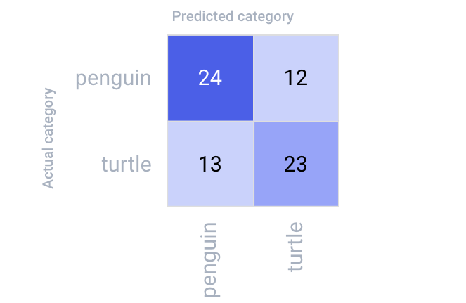
And while this plot is helpful in illustrating a given model’s “confusion” between categories, it only tells part of the story. Are there any patterns in the images the model is struggling with? Maybe the model tends to get confused when it sees a particular breed of one of the animals. Or maybe different backgrounds are influencing its decisions. We really can’t be sure without visualizing exactly what the model predicted, and on which images.
In this article, we’ll explore how to use Comet’s interactive confusion matrix for a multi-class image classification task. Follow along with the full code in this Colab tutorial, and make sure to check out the public project here!
Note that to run these experiments, you’ll need to have your Comet API key configured. If you don’t already have an account, create one here for free.
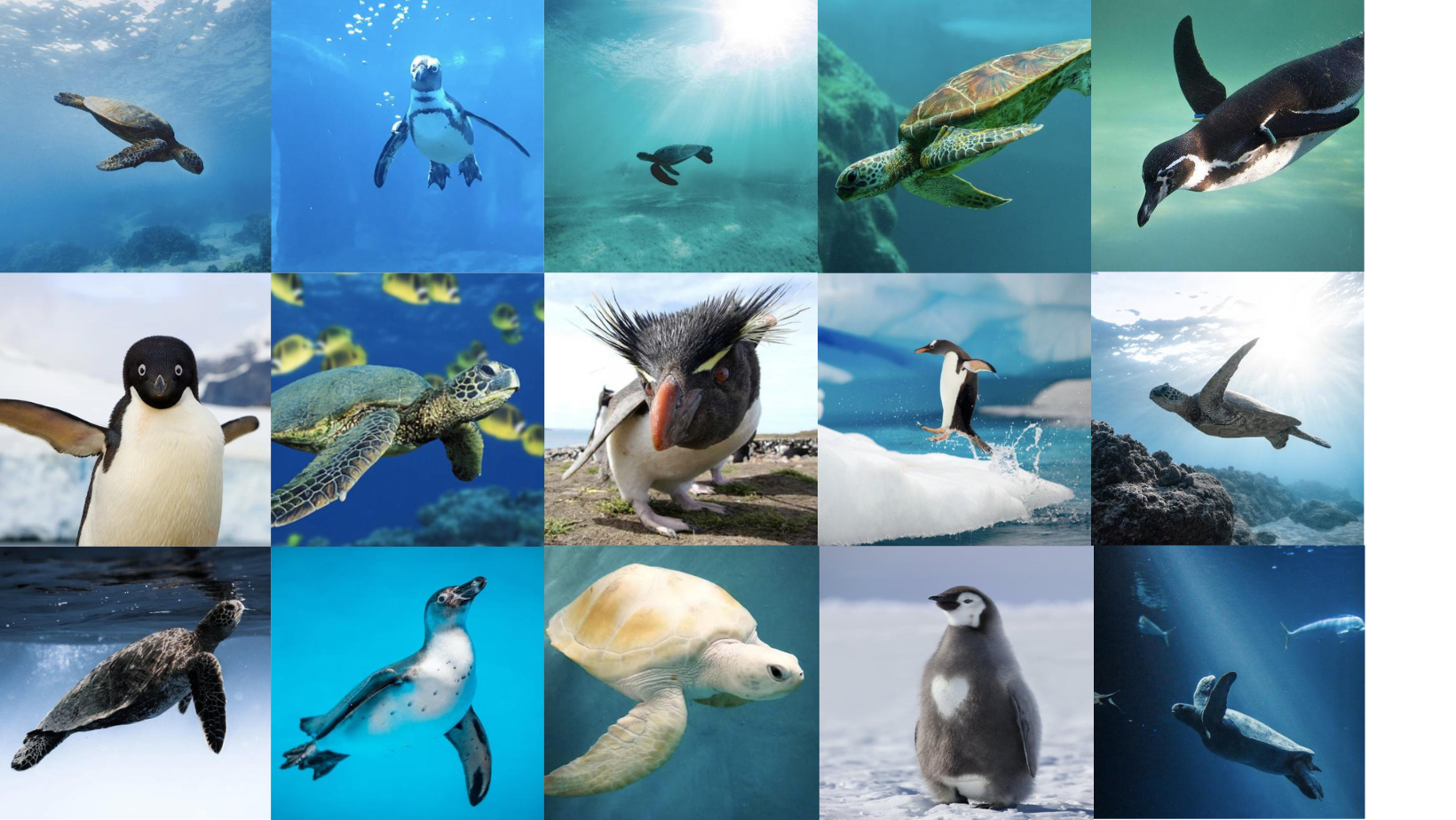
Our Data
For this tutorial, we’ll be using a dataset of 572 images of penguins and turtles.The training set contains 500 images, and the validation set contains 72 images, both of which are split evenly between classes. Each image contains exactly one instance of an object, and since being a penguin, being a turtle, and being the background are all mutually exclusive, this is a multi-class, but not a multi-label classification task. Download the full dataset on Kaggle here and follow along with the code here.
Once we’ve downloaded our dataset, we’ll need to define a custom PyTorch Dataset class to properly load and preprocess our images before feeding them to our model. We’ll also define a label dictionary to convert our categorical labels into numerical ones. Note that by default, our models treat “0” as the background class.
Alternatively, could also choose to one-hot encode our labels before logging them to Comet, as demonstrated in this example notebook.
Finally, we’ll log our hyperparameters to keep track of which ones produce which results:
Training a Classifier
The best object detection models are trained on tens, if not hundreds, of thousands of labeled images. Our dataset contains a tiny fraction of that, so even if we used image augmentation techniques, we would probably just end up overfitting our model. Thankfully, we can use fine-tuning instead! Fine-tuning allows us take advantage of the weights and biases learned from one task and repurpose them on a new task, saving us time and resources in the process. What’s more, fine-tuning often results in significantly improved performance!
We’ll leverage the TorchVision implementation of FastRCNN and MaskRCNN with ResNet50 backbones.
Logging the Interactive Confusion Matrix
Basic Usage
We can log a confusion matrix to Comet in as little as one line of code using experiment.log_confusion_matrix(). Our goal is to visualize how much our model confuses the categories as it trains, that is, across epochs, so we’ll call this method within our training loop. We can then use the final confusion matrix calculated for each experiment run to compare experiment runs across our project. Lastly, we’ll compare what we can learn from our interactive confusion matrix with the images we log to the Image Panel.
Defining a Callback
Alternatively, if we were strictly performing image classification (and not object detection) we could also define a callback to log the confusion matrix. This is the preferred method when logging images to a confusion matrix with a lot of categories because it gives you the option to cache images. By using one image for each image set, and then reusing these between epochs, we can dramatically cut training time.
An example of a confusion matrix callback might look something like this:
For this simple example, however, we’ll calculate and log a fresh confusion matrix at the end of each epoch. This example will create a series of confusion matrices showing how the model gets less confused as training proceeds. Now that we’ve defined the inputs, we can define and log the confusion matrix itself:
Putting it all together
We’ll need to create three lists:
- Ground truth labels (bounding boxes) per epoch
- Predicted labels (bounding boxes) per epoch
- Images overlaid with their respective bounding box predictions per epoch
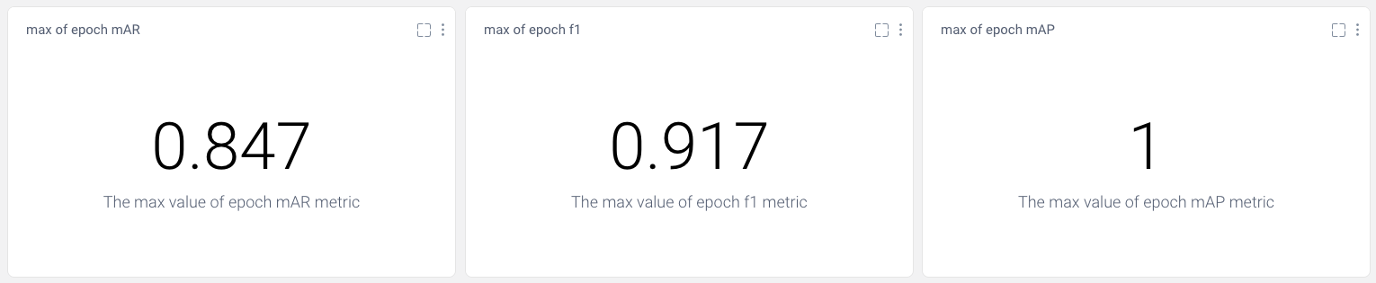
In our example, we’re also going to log our images to the graphics tab to create an image panel in our project view. We’ll also log all of our evaluation metrics to a CSV file and log it as a Data Panel. All together, our training loop will look like this:
Using the Confusion Matrix
View Multiple Matrices
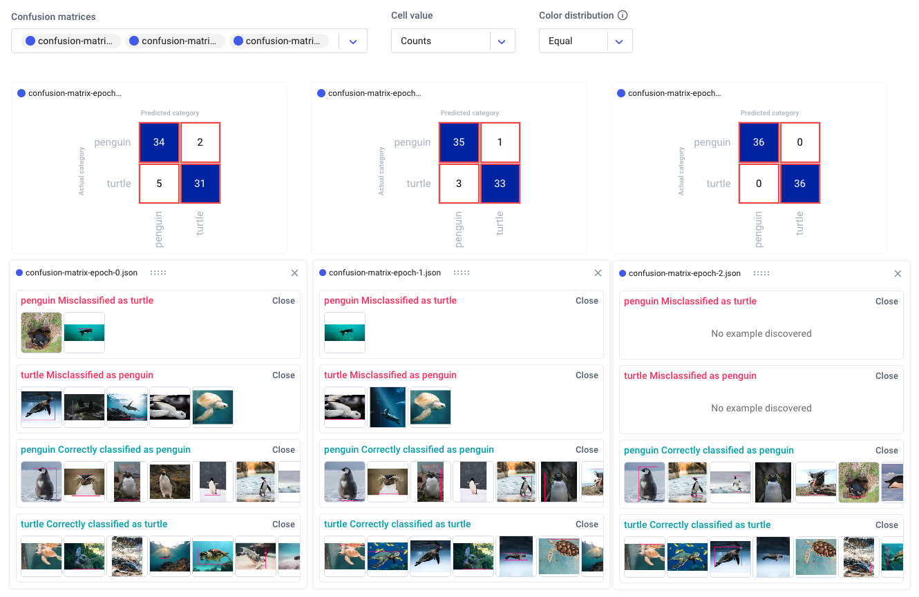
Now we can head over to the Comet UI to take a look at our confusion matrices. Select the experiment you’d like to view, then find the ‘Confusion Matrix’ tab on the lefthand sidebar. We can add multiple matrices to the same view, or switch between confusion matrices by selecting them from the drop-down menu at the top. By hovering over the different cells of the confusion matrix, you’ll see a quick breakdown of the samples from that cell. If we click on a cell, we can also see specific instances where the model misclassified an image. By default, a maximum of 25 example images is uploaded per cell, but this can be reconfigured with the API.
Because we trained our model for three epochs and logged one matrix per epoch, we’ll have three confusion matrices for each experiment run. This will allow us to watch how our models improve over time, while also letting us compare experiment runs across our project. Are there particular images our model tends to struggle with? How can we use this information to augment our training data and improve our model’s performance?
View Specific Instances
In the example below, the model seems to get confused by images of white turtles, so maybe we can add some more examples in a future run. In any event, we can see that our model clearly makes fewer mistakes over time, eventually classifying all of the images correctly.
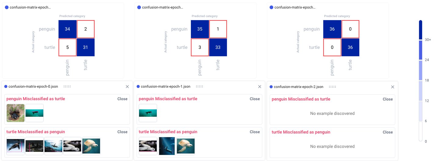
We can also click on individual images to examine them more closely. This can be especially helpful in object detection use cases, where visualizing the bounding box location can help us understand where the model is going wrong.
When examining specific instances of misclassifications, we can see that the model sometimes categorizes large boulders as turtles, and tends to get confused by one particularly unique breed of penguin. We could choose to augment our training data with images containing similar examples to improve performance.
Aggregating Values
We can also choose three different methods of aggregating the cells in our confusion matrices: by count, percent by row, and percent by column. We can further choose either equal or smart color distribution. Equal color distribution divides the range into equal buckets, each with their own color. Smart color distribution ensures that colors are more evenly distributed between cells as the range gets bigger. This second setting can be especially helpful for sparse matrices or matrices with large ranges.
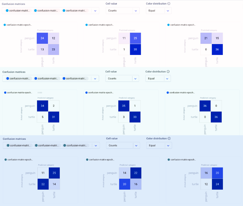
Comparing Experiment Runs
The confusion matrix feature also helps us to compare experiment runs across our project. In the example image below, we show the confusion matrices from three different experiments over three epochs. Each series of confusion matrices gives us a very different picture of how each model is behaving.
Conclusion
Thanks for making it all the way to the end, and we hope you found this tutorial useful! Just to recap everything we covered, we:
- Loaded a multi-class image classification dataset;
- Fine-tuned a pre-trained TorchVision model with our dataset;
- Logged confusion matrices with image examples per epoch, per model;
- Arranged our confusion matrix view and aggregated the values;
- Compared our confusion matrices over time and across multiple experiment runs;
- Used the interactive confusion matrix to debug our image classification model and examine individual instances.
Try out the code in this tutorial here with your own dataset or model! You can view the public project here or, to get started with your own project, create an account here for free!
