
In this article, we’ll leverage the power of autoencoders to address a key issue for banks and their customers: credit card fraud detection. Feel free to follow along with the full code tutorial in this Colab and get the Kaggle dataset here.
Credit Card Fraud
Credit card fraud represents an important, yet complex challenge for banks. In 2021 alone, Nilson estimated that credit card fraud had surpassed $28.5 billion dollars worldwide. And while effective fraud detection efforts, like the use of machine learning and deep learning algorithms, have helped bring about a steady decline in fraud since its peak in 2016, fraud still represents about 6.8% of international credit card transactions.
But fraudulent financial data comes with its own set of unique challenges. Fraudulent transactions represent anomalous data that make up a very small percentage of total transactions. This results in significant class imbalances that make many traditional evaluation metrics, like accuracy, irrelevant.
If you aren’t already, you can follow along with the full code in this Colab.
The Data
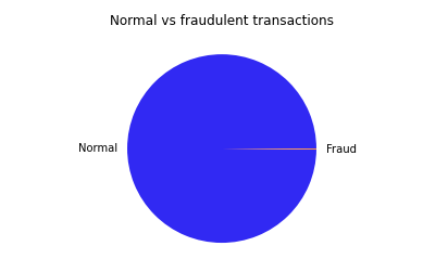
Our data consists of two days’ worth of real bank transactions made by European cardholders in 2013. In this dataset, fraud makes up just 0.172% of all transactions, meaning a model that predicted “no fraud” for every single observation would still achieve an accuracy of over 98%! In the pie chart below, fraudulent transactions are represented by the tiny orange sliver.
Additionally, in order to protect all personal identifiable information (PII) in this dataset, all features (besides Time and Amount) have undergone a PCA transformation. This means that we cannot use any domain knowledge for the purposes of feature engineering or selection.
Data Visualization and Pre-processing
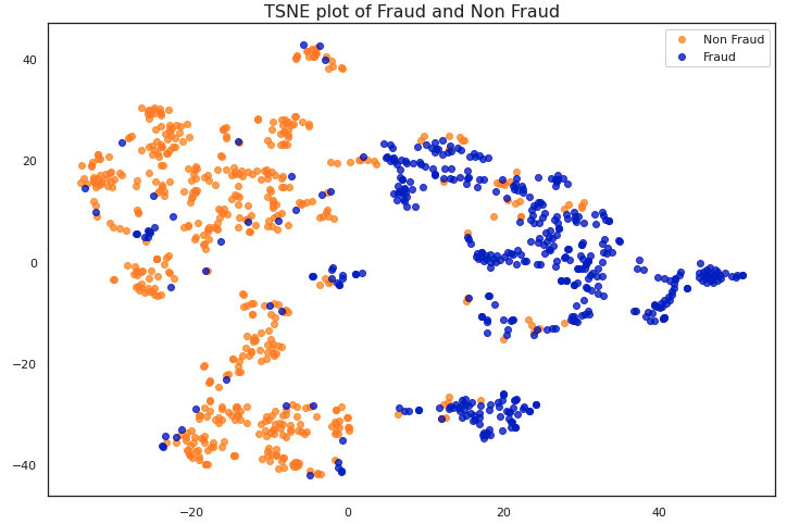
Let’s start out by visualizing our data. It would be impossible to plot 30 dimensions, so first we’ll apply Scikit-Learn’s implementation of t-SNE to the data. t-SNE is a dataset decomposition technique. Here we only plot the first two components with maximum information.
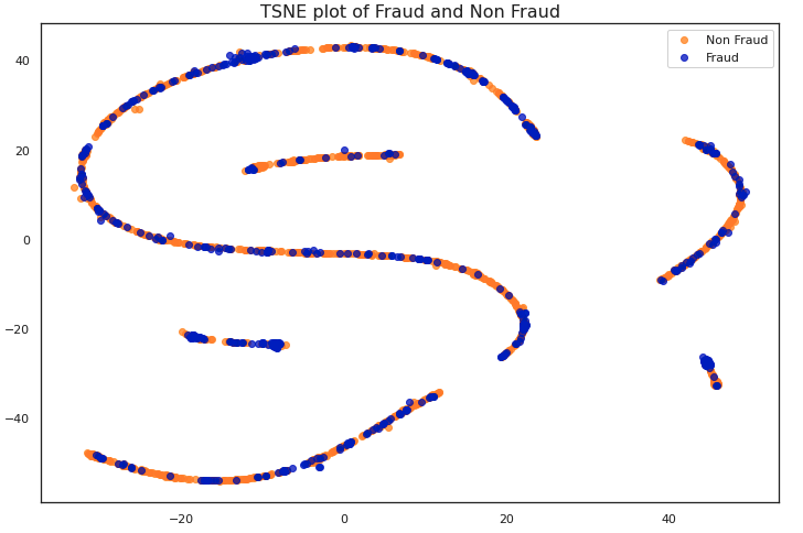
We can observe in this graph that there is little difference between fraudulent and non-fraudulent transactions. Most machine learning models would struggle to classify this data as-is.
First, we’ll perform some very basic transformations to the data before feeding it to our model. The original Time feature represents the number of seconds elapsed between each transaction and the first transaction in the data. We’ll convert this relative time measure to hour-of-the-day.
We also scale the Time and Amount features, as all other features (V1, V2, … V28) were previously scaled during the PCA transformation. Finally, because we are training an autoencoder to “learn” the embeddings of a normal transaction, we’ll subset just normal samples as our training dataset, and use a 50:50 split of normal and fraudulent samples for our validation set. We’ll also set aside 250 samples for a test dataset of completely unseen data.
Attacking Data Imbalance With Autoencoders
Due to the stark class imbalances in this dataset, for this challenge we will use an Autoencoder. Autoencoders learn an implicit representation of normality from the “normal” samples, allowing us to reserve our sparse fraudulent data samples for testing. During inference, new samples are compared against the embeddings of normal samples to determine whether or not they are fraudulent.
Model Training and Inference
We define a simple Autoencoder model with two fully connected linear layers and the Tanh activation function. We’ll be using mean squared error as our loss function and an Adam optimizer. We’ll log all of this information to Comet, an experiment tracking tool, so we can compare how different experiment runs performed later on.
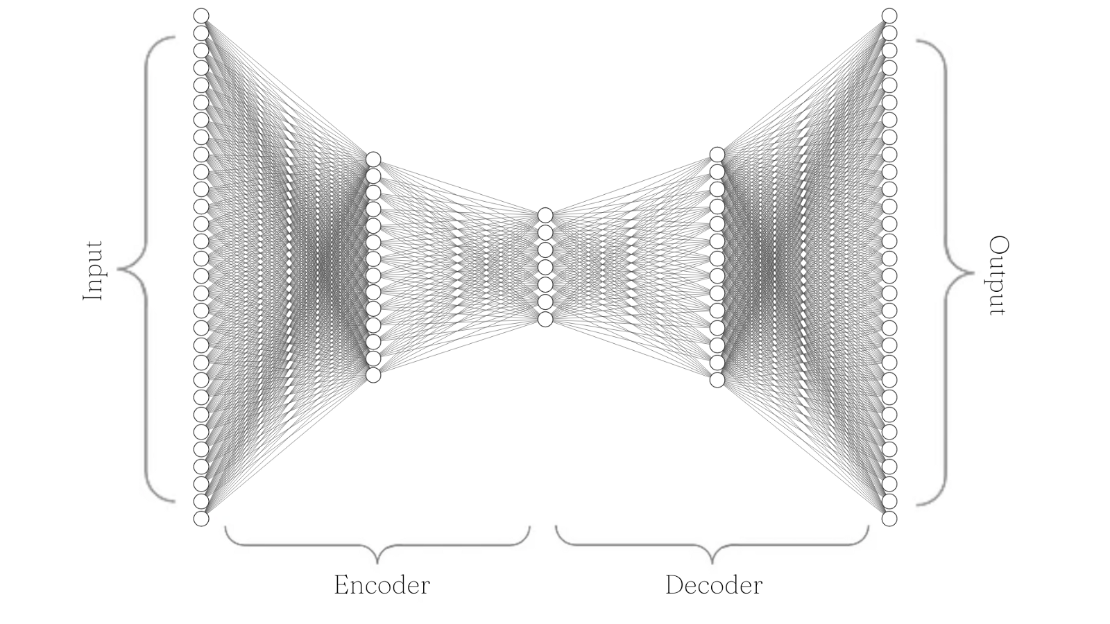
We can quickly visualize this model architecture with the following diagram. Note that we start with 30 input nodes, then encode this information down to seven nodes, and then decode back to 30 output nodes.
Next, we define our training and validation loops. Note that we create our val_predictions table by defining a pandas DataFrame within our validation loop and appending the relevant columns. We’ll use this DataFrame to examine sample-level metrics in Comet after inference.
Precision-recall Curve vs Threshold Values
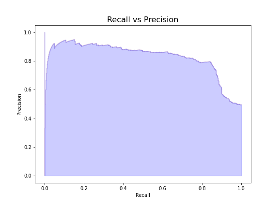
Now that we’ve run training and validation loops, let’s examine the precision-recall tradeoff of our model at various threshold levels and plot the reconstruction error against our chosen threshold. To see how we defined our custom plotting functions, see the Colab here.
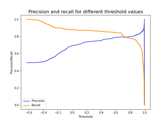
From the plot above, we can see the optimal threshold value for fraudulent transactions is around 0.75. Now let’s plot the precision-recall tradeoff of the model with the threshold set to this value.
Visualizing Reconstruction Error of Credit Card Fraud
Finally, let’s visualize the reconstruction error with the threshold level applied to see how well it separates fraudulent transactions from non-fraudulent transactions.
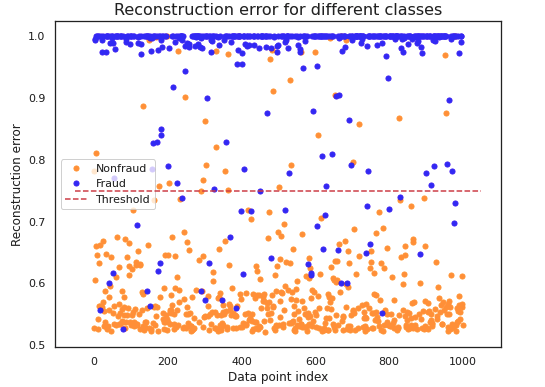
Although some outliers are still misclassified, the threshold separates the vast majority of the reconstructed labels. Note that we used a 50:50 split of fraudulent and non-fraudulent data for the validation split.
To get a better understanding of how our autoencoder has learned to distinguish between the two classes, let’s visualize plots of the raw data (before encoding) and the transformed data (after reconstruction). Here again, we’ll apply t-SNE to each dataset and plot the first two components with maximum information.
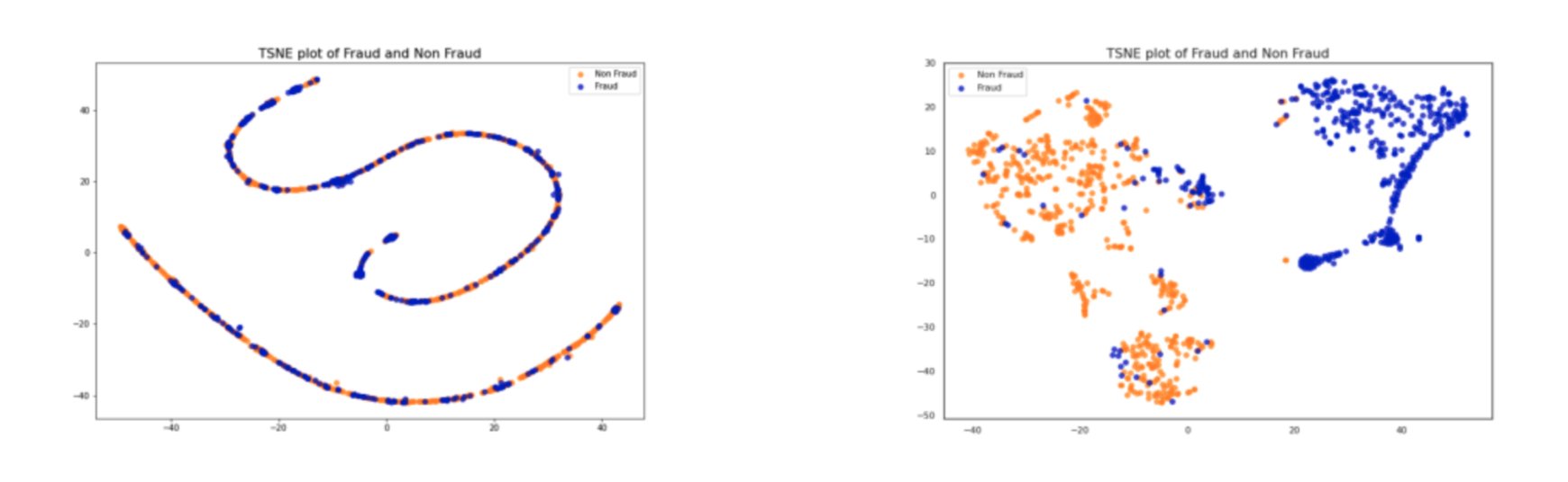
Clearly the data on the right is much easier to separate (and therefore classify), than the data plotted on the left. It would be very difficult for a machine learning algorithm to classify the data on the left at all, so our autoencoder has proven very helpful.
Classification Report and Evaluation
Let’s also take a look at the classification report of our validation data. Note that although the original dataset was highly imbalanced, we made a validation set that was roughly equally split between normal and fraudulent transactions. This gives our model a better opportunity to predict both classes, and also makes the evaluation metrics much more relevant.
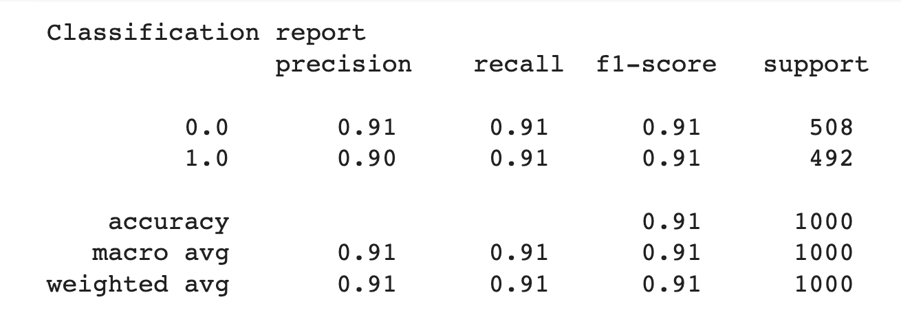
With a precision, recall, and F1-score of 0.91, our model has done well! But can we do any better? Let’s take a look at the data we logged to Comet to identify where our model might be improved. We can also check out how to monitor testing data statistics as our model gets a chance to look at new, unseen data.
Debugging Our Fraud Detection Model With Data Panels
Once we’ve run training and inference, we can head over the Comet UI to check out our Data Panels. Follow along with my public project here and feel free to experiment with customization options like join types, column order, and more. We’ll also take a peek at how to filter and sort the Data Panel to identify misclassified samples for retraining.
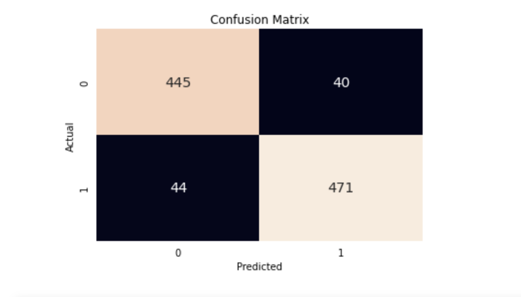
Data Panels are interactive so we can filter samples based on the ground truth labels and compare them to the model’s predictions. Since not detecting fraudulent cases when they are actually occurring could potentially cost financial institutions a lot of money, we specifically want to look at instances where there was fraud, but the model predicted there wasn’t (false negatives).
We can also gather all instances where the model predicted there was fraud but there wasn’t (false positives). By re-training the autoencoder on these problematic samples, we can improve the model’s representation of “normality” for future runs.
We can also track how prediction columns are changing for the same samples across experiments. By concatenating the tables via columns, we can see side-by-side how our predictions compare to previous runs.
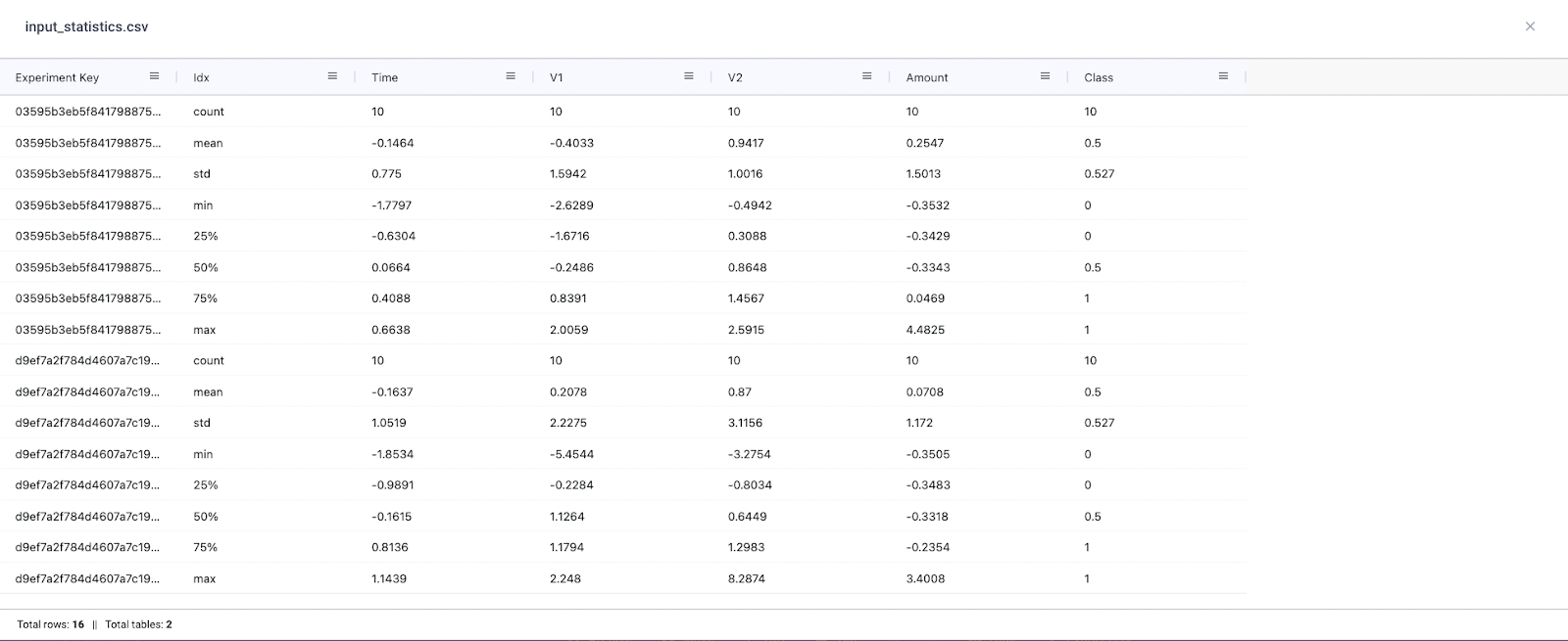
Finally, we can also compare distribution shifts in the input data. If we were using different versions of data across experiments or running experiments over time, it would be a good idea to log some basic summary statistics (like those calculated with pd.df.describe) of the input data. This will allow us to quantify the statistical differences between data and whether this is having a substantial impact on model performance.
Conclusion
Thanks for making it all the way to the end and we hope you found this tutorial useful! To recap everything we’ve accomplished, we:
- Loaded a notoriously imbalanced dataset
- Constructed a simple Autoencoder model
- Plotted reconstruction labels and defined a classification threshold
- Calculated validation metrics
- Logged sample and project-level data to Comet, an experiment tracking tool
- Examined specific instances where the model struggled and identified areas for improvement
