Introduction
Object detection is one of the most popular applications of machine learning for computer vision. A detection model predicts both the class types and locations of each distinct object in an image. Object detection models have a wide range of applications including manufacturing, surveillance, health care, and more.
TorchVision is a Python package that extends the PyTorch framework for computer vision use cases. In TorchVision’s detection module, developers can find pre-trained object detection models that are ready to be fine-tuned on their own datasets. But how can you systematically find the best model for a particular use-case? Here, we’ll explore how to use an experiment tracking tool like Comet to visually compare and evaluate object detection models.
Follow along with the full code in this Colab and check out the public project here!
What is Object Detection?
Object detection is a computer vision task that aims to identify instances of objects in images and assign them to specific classes. At a low level, object detection seeks to answer the question, “what objects are where?”

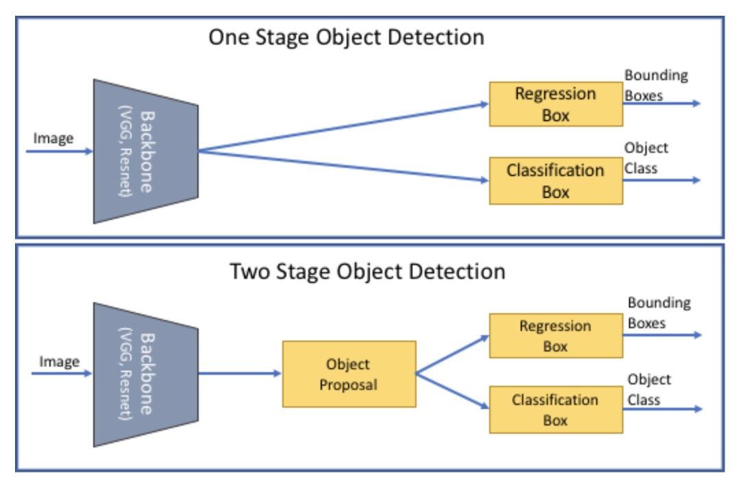
Object detection algorithms are generally separated into two categories: single-stage (RetinaNet, SSD, FCOS, YOLO, etc.) and two-stage (Fast RCNN, Mask RCNN, FPN, etc.). In two-stage detectors, one model is used to extract generalized regions of objects, and a second model is used to classify and further refine the location of an object. Single-stage detectors do all of this in one step. Single-stage detectors tend to be faster and less computationally expensive than two-stage detectors, but they’re also less accurate.
Finetuning Pre-trained Models
The best object detection models are trained on tens, if not hundreds, of thousands of labeled images. What’s more, image datasets themselves are inherently computationally expensive to process. To train an object detection model from scratch requires a lot of time and resources that aren’t always available. To train several object detection models for comparison requires even more time and resources. Thankfully, we don’t have to. Instead, we can use transfer learning or fine-tune pre-trained models.
In essence, both these methods allow us to take advantage of the weights and biases learned from one task and repurpose them on a new task. By leveraging feature representations from a pre-trained model, we don’t have to train a new model from scratch, saving us time and compute resources. What’s more, these methods can contribute to rapid boosts in model performance for little overhead.
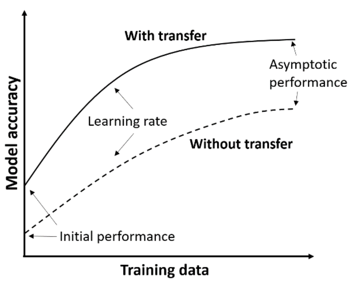
Transfer learning and fine-tuning are similar processes but with one key difference. In transfer learning, all previously trained layers are frozen, and (optionally) additional layers are added for retraining. In fine-tuning, all previously trained layers are retrained, but at a very low learning rate. Both methods typically result in boosted initial performance, steeper improvement slopes, and elevated final performance.
TorchVision’s Pre-Trained Models
In real-world applications, we often make choices to balance accuracy and speed. The performance of a model under a given set of circumstances might not be relevant if we aren’t able to replicate those circumstances in production. So when looking for the “best” object detection model, it becomes essential to monitor a wide range of metrics pertaining your particular use case. In this tutorial, we’ll show you how Comet helps us do this.
TorchVision’s detection module comes with several pre-trained models already built in. For this tutorial we will be comparing Fast-RCNN, Faster-RCNN, Mask-RCNN, RetinaNet, and FCOS, with either ResNet50 of MobileNet v2 backbones. Each of these models was previously trained on the COCO dataset. We will download the trained models, replace the classifier heads to reflect our target classes, and retrain the models on our own data.
Image Data Formats
In computer vision, images are represented as matrices of pixel intensity values. Black and white (grayscale) images are usually two-dimensional, and color images are typically three-dimensional, with one “layer” each representing red, blue, and green pixels.
Just as there are several ways to represent images, there are also several ways we can represent our labels and predictions. In the full code for this tutorial, we’ll provide methods for logging bounding boxes, segmentation masks, and polygon annotations to Comet. But when comparing our TorchVision models we will only use bounding boxes, as not all of our models are able to calculate the other types of predictions.
To further complicate things, not all algorithms format bounding box annotations in the same way. Below we’ve listed a few of the most common bounding box formats you’re likely to run into, but we’ll be focusing on Pascal VOC and COCO formats in this tutorial.
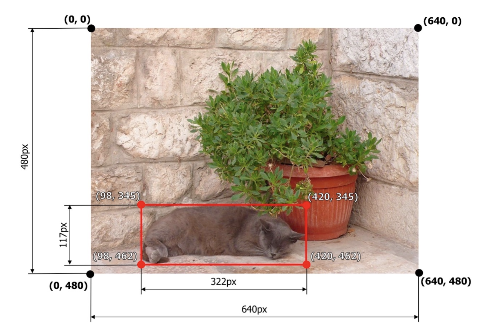
Pascal VOC: [xmin, ymin, xmax, ymax] → [98, 345, 420, 462]
Albumentations: normalized([x_min, y_min, x_max, y_max]) → [0.153125, 0.71875, 0.65625, 0.9625]
COCO: [xmin, ymin, width, height] → [98, 345, 322, 117]
YOLO: normalized([x_center, y_center, width, height]) → [0.4046875, 0.8614583, 0.503125, 0.24375]
Evaluation Metrics for Object Detection
A naive approach to evaluating object detection models might be binary classification (“match” or “no match”, “1” or “0”), but this method leaves little room for nuance. We can do better!
Intersection Over Union (IOU)
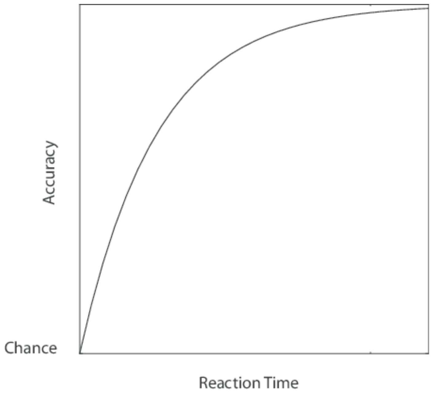
The standard evaluation metric for comparing individual bounding boxes is Intersection over Union, or IoU. IoU evaluates the degree of overlap between the ground truth bounding box and the predicted bounding box with a value between 0 and 1.
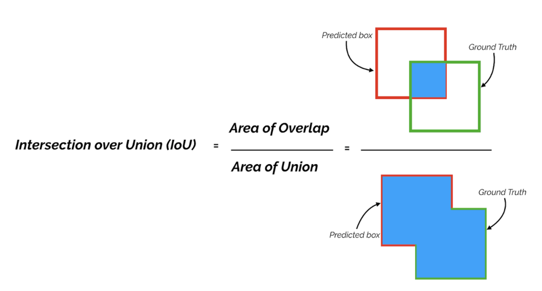

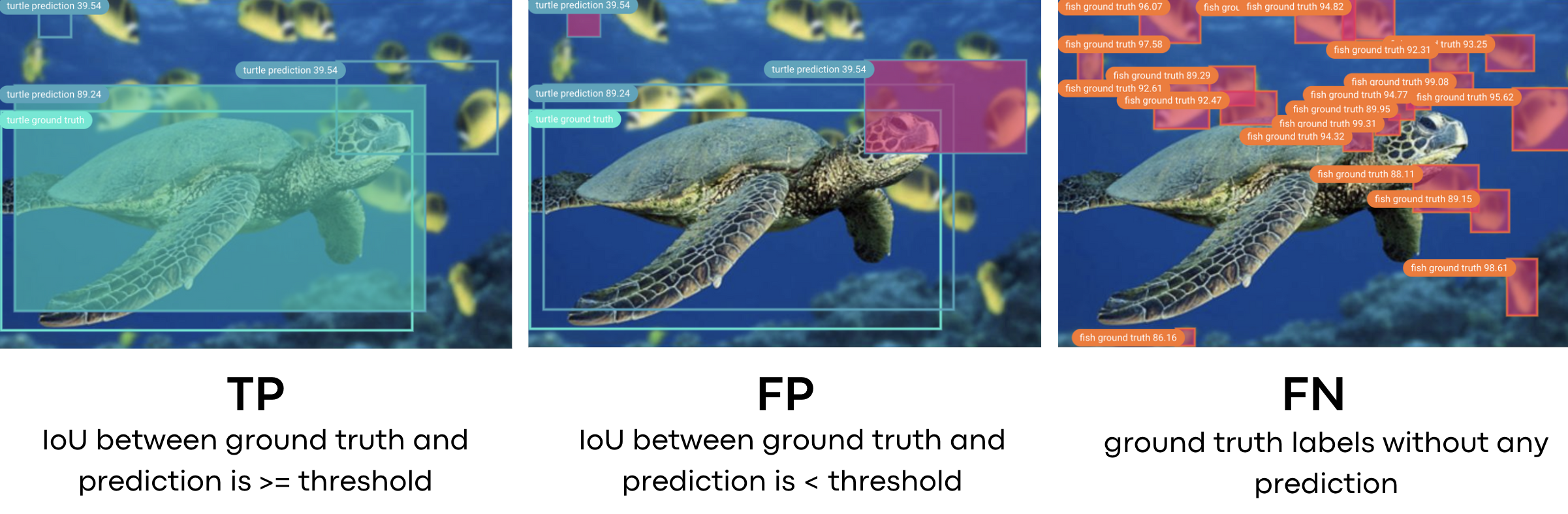
IoU is determined for each set of bounding boxes in an image and then a threshold is applied. If an IoU meets the threshold, it’s marked as a “true positive.” All predictions not marked as “true positives” are marked as “false positives,” and any items left in our “ground truth” annotations list are marked as “false negatives. The decision to mark a detection as TP, FP, or FN is completely contingent on the choice of IoU threshold. The IoU threshold is commonly set at 0.5, but you may want to experiment with this number. Once we’ve calculated our confusion matrix, we can compute precision and recall.
Mean Average Precision (mAP) and Mean Average Recall (mAR)
Precision (also known as specificity) is the degree of exactness of the model in identifying only relevant objects. The equation for precision is:

Recall (also known as sensitivity) measures the ability of the model to detect all ground truths. The equation for recall is:

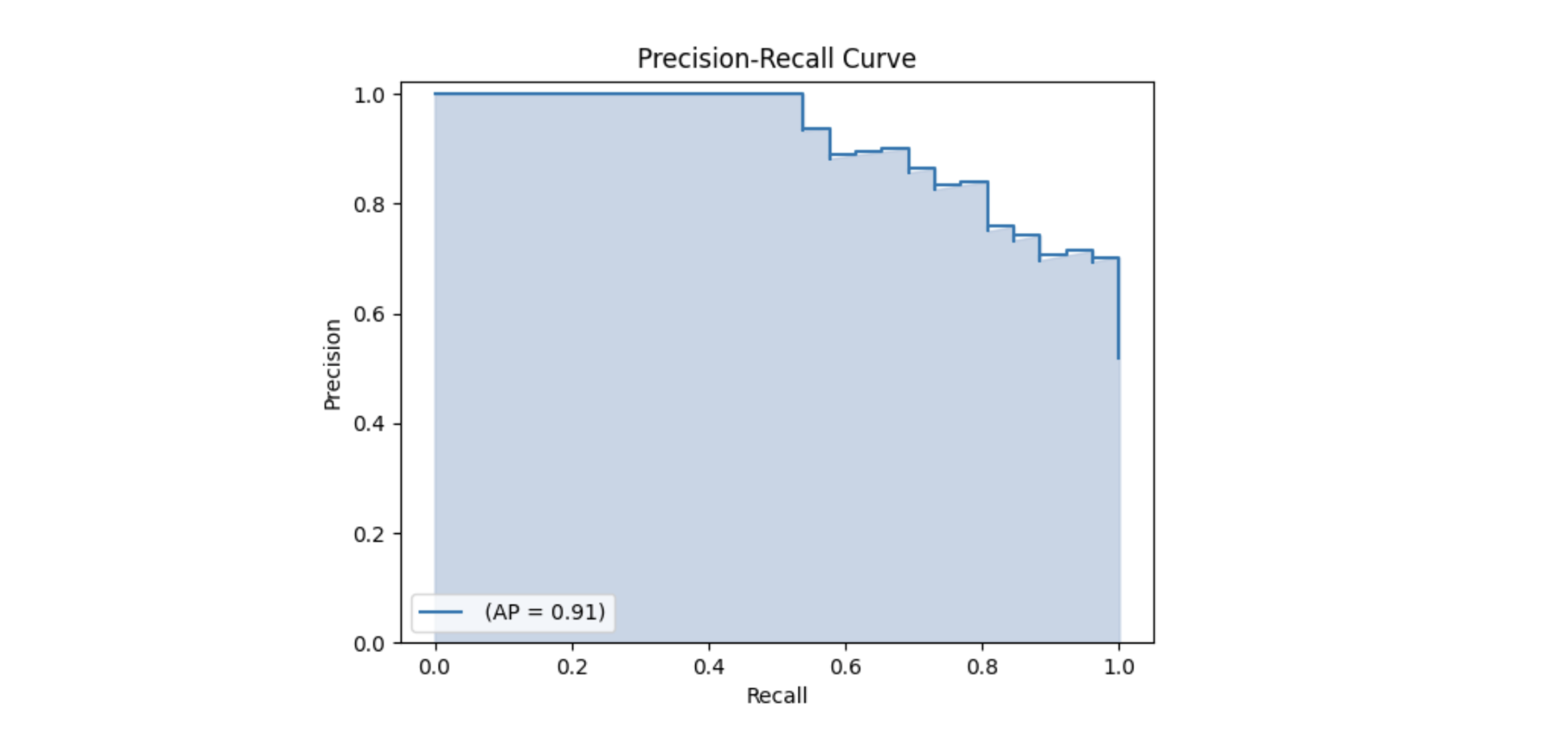
In a perfect world, our perfect model would have a precision and recall of 1, meaning it predicted zero false negatives and zero false positives. But in the real world this isn’t generally achievable. A precision-recall curve plots the value of precision against recall for different confidence thresholds. The area under this curve is also referred to as the Average Precision (AP). Average recall (AR) describes double the value of the area under the recall-IoU curve.
Mean Average Precision (mAP) and mean Average Recall (mAR) are calculated by taking the weighted mean of the AP or AR over all classes and/or over all IoU thresholds. They are two of the most common evaluation metrics for object detection and are used to evaluate submissions in popular computer vision competitions like the COCO and Pascal VOC challenges. We can derive many other metrics from mAP and mAR, including mAP across scales, at different IoU thresholds, and with a minimum number of detections per image.
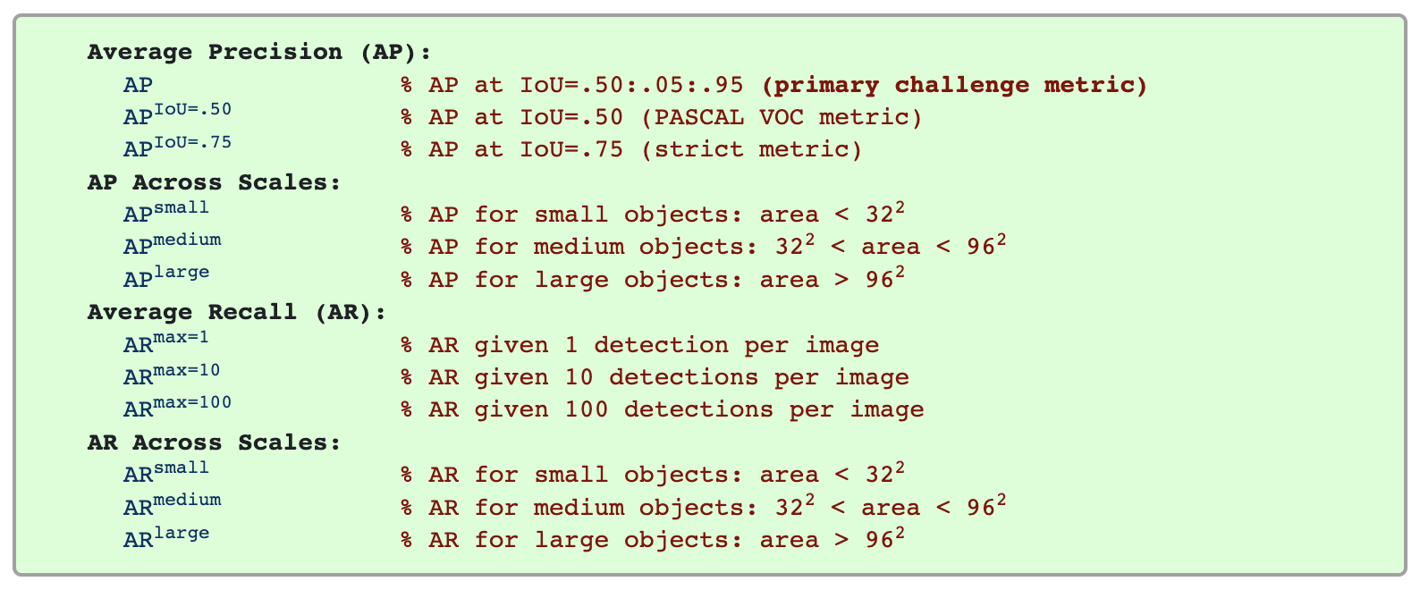
Other metrics
If we were building a model to detect very large objects (relative to the image’s field of view), we might be willing to consider models with poor “AP_small” scores, as this metric would be less relevant to our use case. If we were planning on using our model to aid in medical diagnoses, we might place a higher emphasis on mAR values than mAP values, since it would likely be more important not to miss any positive samples than it would be to miss negative samples.
For this tutorial we use a combination of the mAP and mAR values calculated by the COCO evaluator and torchmetrics.detection module. We’ll log all relevant values to a DataFrame and then examine it more closely in the Comet Data Panel. This will help give us a full picture of how different models perform in different scenarios and we’ll choose our “best” model accordingly.
Challenges of Comparing Object Detection Models
Comparing object detection models can be challenging for a number of reasons. Different models have different requirements when it comes to input size and shape, annotation formats, and other dataset attributes. Hyperparameters vary from algorithm to algorithm and keeping track of which values produce which results can quickly become tedious and overwhelming.
Most computer vision pipelines incorporate image augmentation in some form, so dataset versioning becomes essential for reproducibility and explainability. What’s more, performance metrics only tell part of the story when it comes to object detection. Often, it’s necessary to visualize prediction annotations to understand where things are going right– and where they’re going wrong.
What’s more, image datasets themselves are inherently computationally expensive to process. To train an object detection model from scratch requires a lot of time and resources that aren’t always available. To train several object detection models for comparison requires even more time and resources.
In real-world applications, we often make choices to balance accuracy and speed. The performance of a model under a given set of circumstances might not be relevant if we aren’t able to replicate those circumstances in production. So when looking for the “best” object detection model, it becomes essential to monitor a wide range of metrics pertaining your particular use case. In this tutorial, we’ll show you how Comet helps us do this.
Using Comet for Object Detection
Clearly, comparing object detection models isn’t nearly so simple as just minimizing a single loss function. We have a pretty wide range of metrics to calculate and log, some of which need to be visualized to completely understand, and each model has it’s own graph definition, set of hyperparameters, code output, and other features. To help keep track of all of these moving pieces, we’ll log our inputs, metrics, and outputs to Comet, a experiment tracking tool. Comet has some pretty extensive auto-logging capabilities, but we’ll also explore how to log custom metrics and outputs to Comet. By visualizing all of our data in the Comet UI, we’ll be able to get a much more complete understanding of how each of our models behaves, under which circumstances, and with which data.
For this tutorial, we’ll be using the Penn-Fudan dataset, which consists of 170 images labeled with 345 instances of pedestrians. Pedestrian detection has several applications, including surveillance, training self-driving cars, and other traffic safety applications. Since we’re using PyTorch, we’ll need to define a custom dataset class that inherits from the torch.utils.data.Dataset class.
All of the models in TorchVision’s detection module use Pascal VOC format, so we’ll format our bounding boxes accordingly. We’ll then need to convert the model’s prediction labels from Pascal VOC to COCO format for use with the COCO evaluator and Comet. If you’re using this tutorial with your own model, check your specific model’s annotation requirements.
Single Experiment View
In order to get a good understanding of how each of our models is performing, and with which hyperparameters, we’ll start by examining our results at an experiment-level.
Store Hyper-parameters
Keeping track of our hyperparameters is essential for reproducibility and explainability. Model hyperparameters can affect model performance, computational choices and what information to retain for analysis. Hyperparameters vary from algorithm to algorithm, and some are more important than others, so this critical task can quickly become tedious and confusing.
Here, we log important hyperparameters with just a single command. For our project we’ll be monitoring the following hyperaparameters, which we can adjust by simply editing the relevant keys-value pairs:
Sometimes metrics that work well for one model may not work at all for another. For example, the FCOS model tends to struggle with exploding gradients. When using it, we have to significantly decrease the learning rate to accommodate for this. If, however, we use the reduced learning rate on a model like Fast-RCNN, (typically one of our best-performing models), it performs unusually poorly. This is because it fails to ever really “learn” the feature maps of our dataset.
Since we are focusing on comparing different models in this tutorial, we will mostly be keeping the hyperparameters constant. However, if we were looking to optimize the hyperparameters of a single model, we could also pass a list of values to each key and use an optimizer to iterate through them. Comet has a built-in optimizer that supports RandomSearch, GridSearch, Bayes’ Optimization, and custom-built optimization algorithms.
Visualizing Outputs
System Metrics
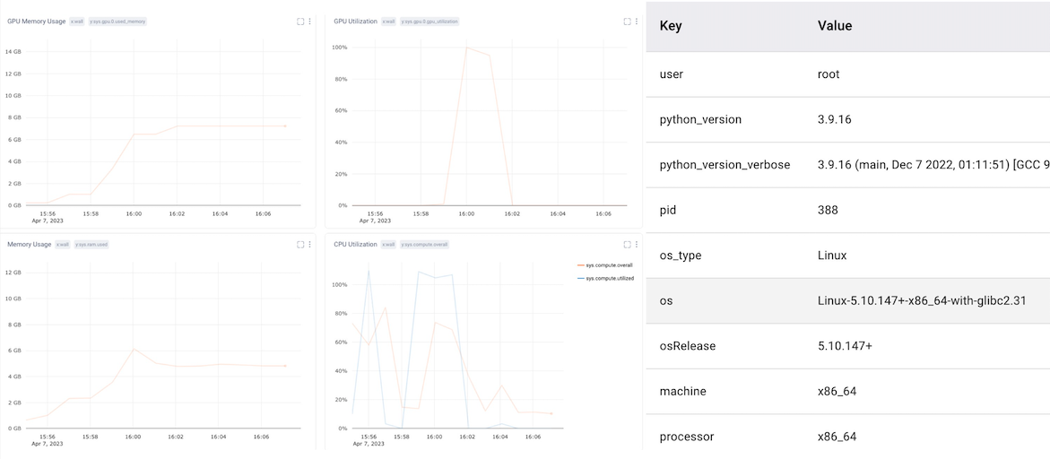
Since object detection is such a resource-heavy task, we’ll also want to monitor our system metrics, including CPU and GPU usage. Luckily, Comet automatically does this for us, so we don’t need to add any additional code. This can also help diagnose bottlenecks in our pipeline, aid with reproducibility, and debug crashed experiments.
Evaluation Metrics
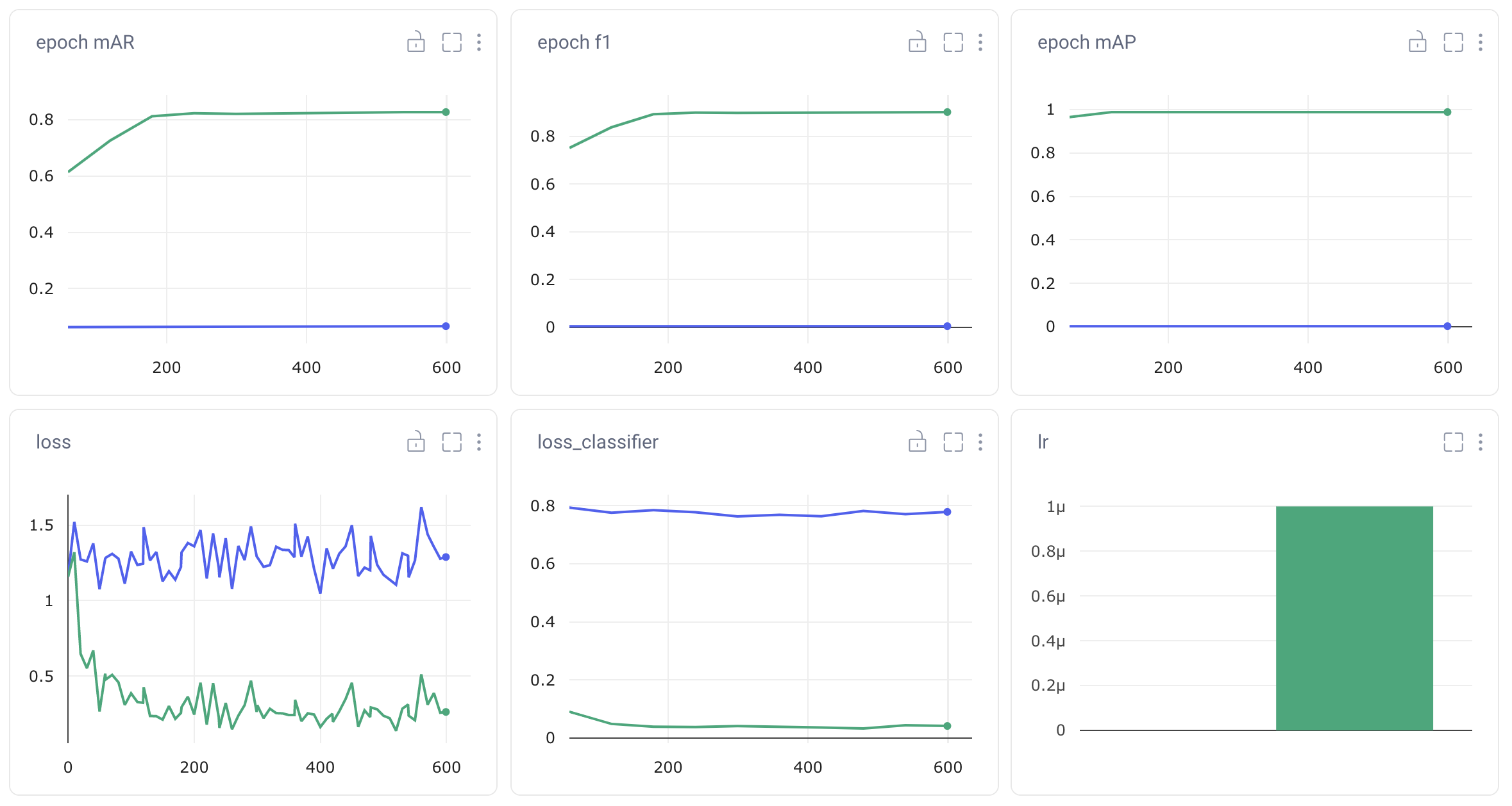
Each of our PyTorch detection models comes with relevant evaluation metrics built-in. Comet’s is integrated with PyTorch, so each of these pre-defined metrics will be automatically logged to the experiment. This is very helpful when comparing multiple runs of the same model, or different object detection models with the same evaluation metrics, but the PyTorch models we’ve chosen don’t all come with the same built-in metrics. We’ll still use these auto-logged plots to get an initial impression of the performance of our models, but we’ll want to log some of our own metrics for cross-experiment comparisons.
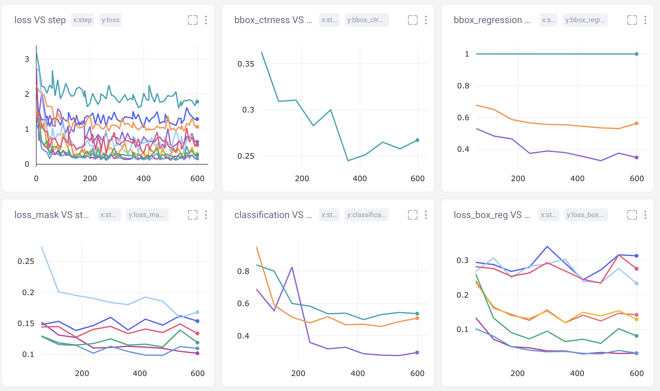
We have the ability to manually log just about any metric, asset, artifact, or graphic we want. In this tutorial, we’ll track:
- Mean Average Precision (mAP) of all validation images per epoch
- Mean Average Recall (mAR) of all validation images per epoch
- Torchmetric’s 12 metrics for characterizing the performance of an object detection (very similar to COCO’s 12 metrics listed above) per image
- Relevant code files from torchvision (engine.py, transforms.py, etc.)
- Graph definitions of our various models
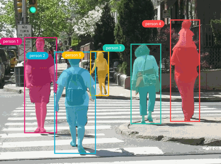
- Each image in the validation dataset, as well as our model’s predicted bounding boxes, with their corresponding labels and confidence scores.
Graphics Tab
Understanding where your model is going right and where it’s going wrong can be especially difficult with image datasets. Loss metrics and other scalar values don’t always tell the whole story and can be hard to visualize. So we’ll also log each of our validation images, along with their predicted bounding boxes, per model per epoch. Flipping through a model’s predictions can also be helpful to see how our models improve over time.
To log images to Comet, we simply use the ‘log_image’ method:
Alternatively, we can also pass the annotations to the metadata parameter:
In either case, the image annotations should be in JSON format and the bounding boxes should be in COCO format. Bounding boxes can either be passed as a dictionary (as shown below) or as a list of lists. Note that a new instance should be created for each bounding box. Polygon points are passed in the format [x1, y1, x2, y2, …, xn, yn].
Project Level View
Since we’re comparing object detection models in this tutorial, one of the most important ways we can use Comet is to create a holistic project-level view. Comet automatically generates a basic model performance panel, but we also have the ability to customize our panels for our particular use case.
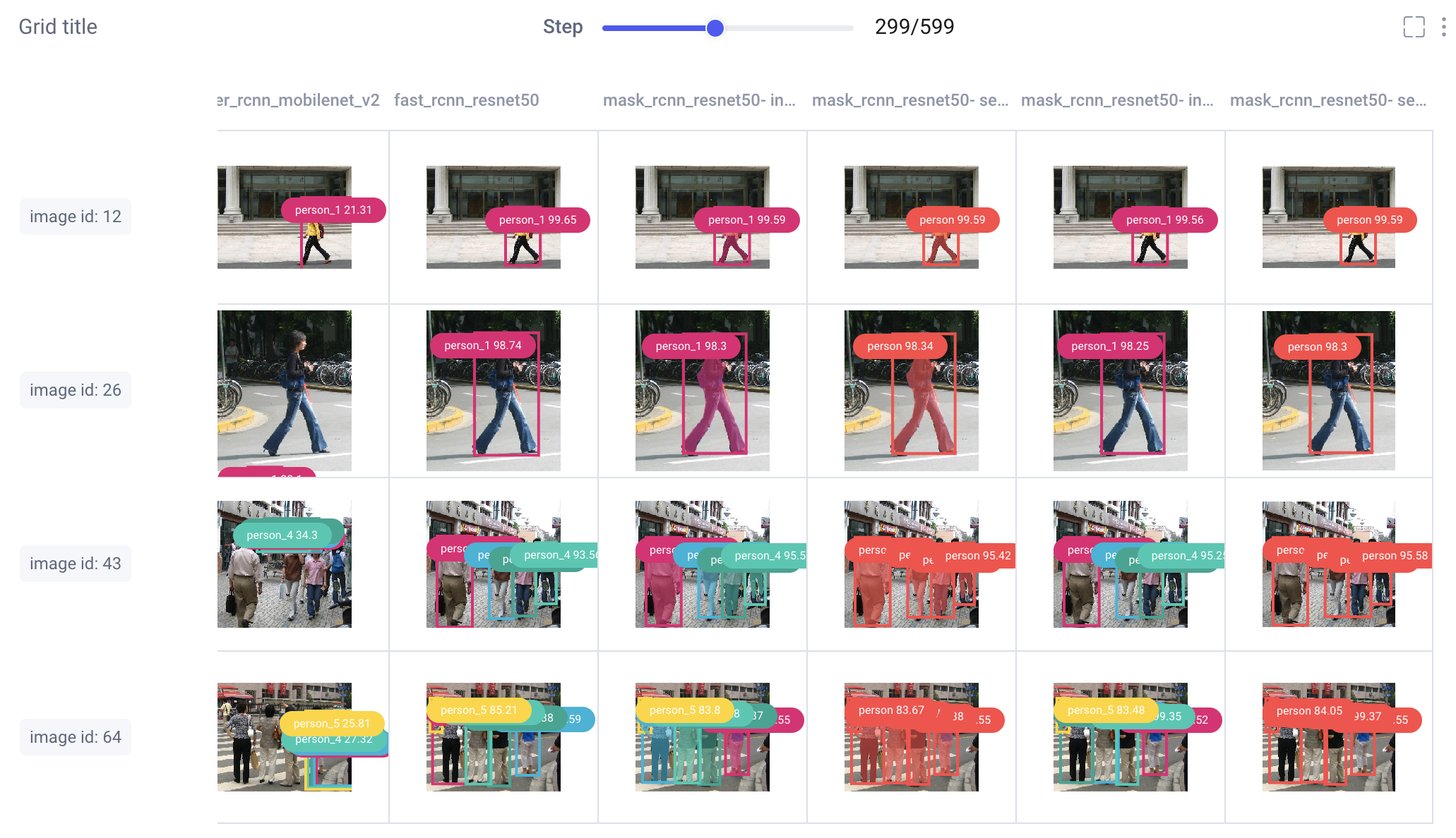
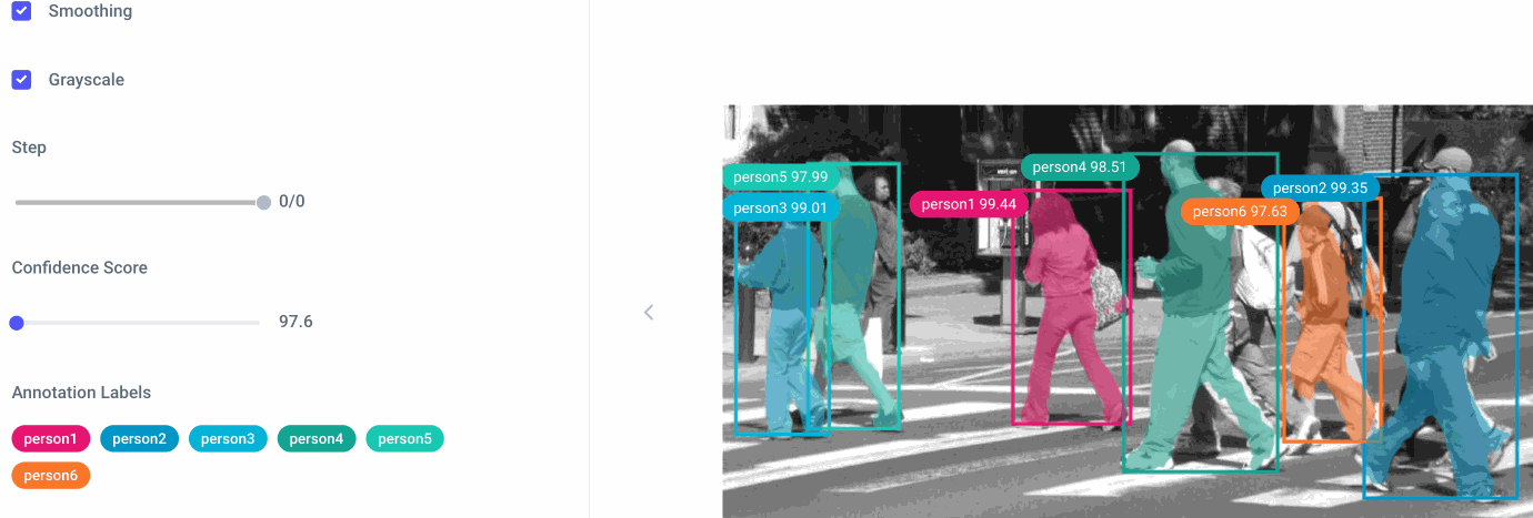
Image Panel
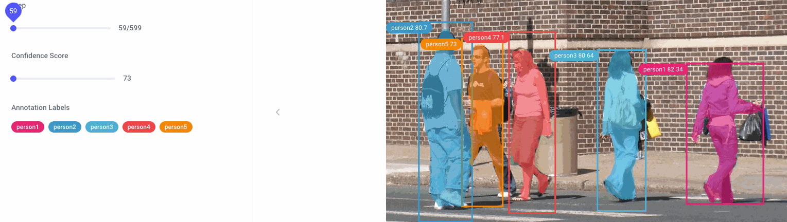
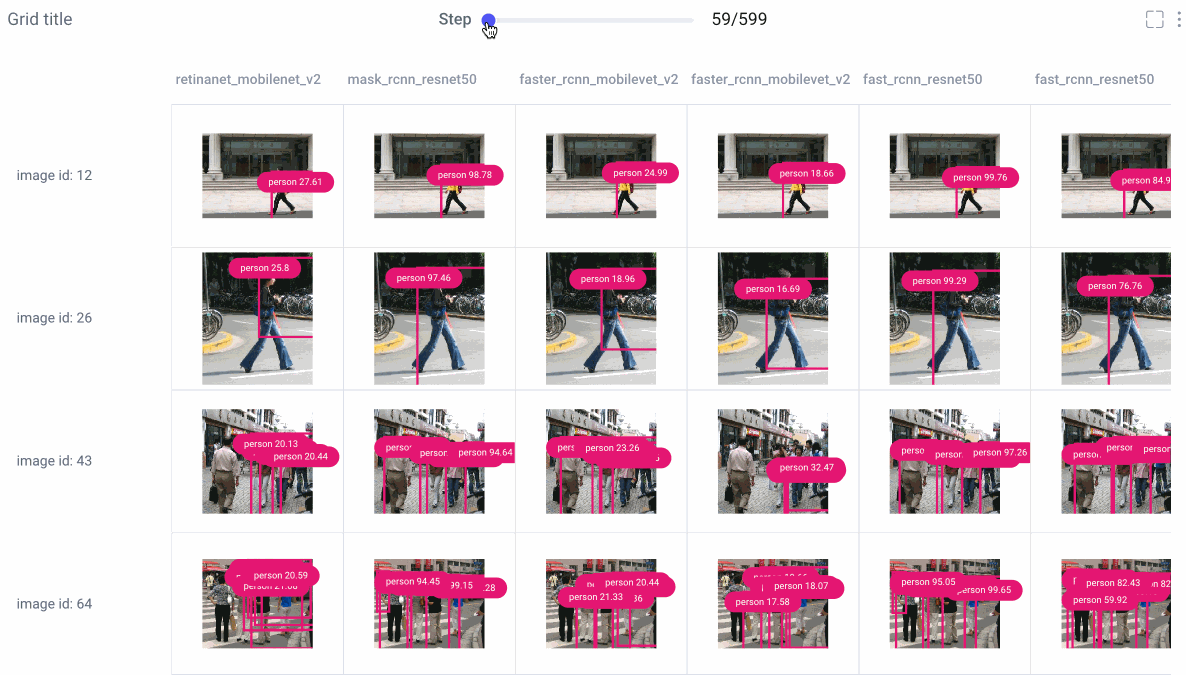
Comet’s new image panel allows us to visualize different models’ prediction per experiment run, over time. Use the step slider to walk through each model’s predictions, or click on an individual image for a closer look.
From there, choose to smooth your image or render it in grayscale, select which class labels you want to examine, and set confidence thresholds with a sliding bar.
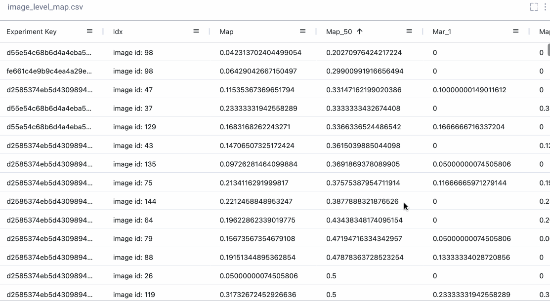
Data Panel
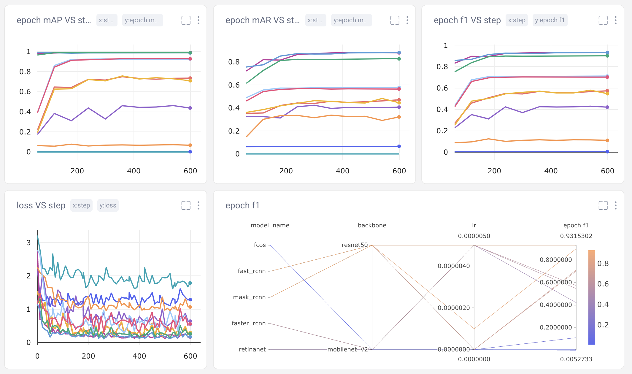
Sometimes we really want a deep dive into the numbers. With Comet’s Data Panel we can log any CSV, DataFrame or table to our project and explore it interactively in the UI. We logged all 12 evaluation metrics from TorchMetric’s mean_ap module, as shown below. A prediction receives a score of -1 if a given metric isn’t relevant to that particular image. For example, if an image doesn’t predict any “large” bounding boxes, then mAP_large for that image will be -1. We can reorder columns, sort them, and filter values. Below, we compare our most basic mAP and mAR measures and then sort them to see where precision is very different from recall. Alternatively, we could also check the epoch f1-score that we logged as an additional tool in our toolbox.
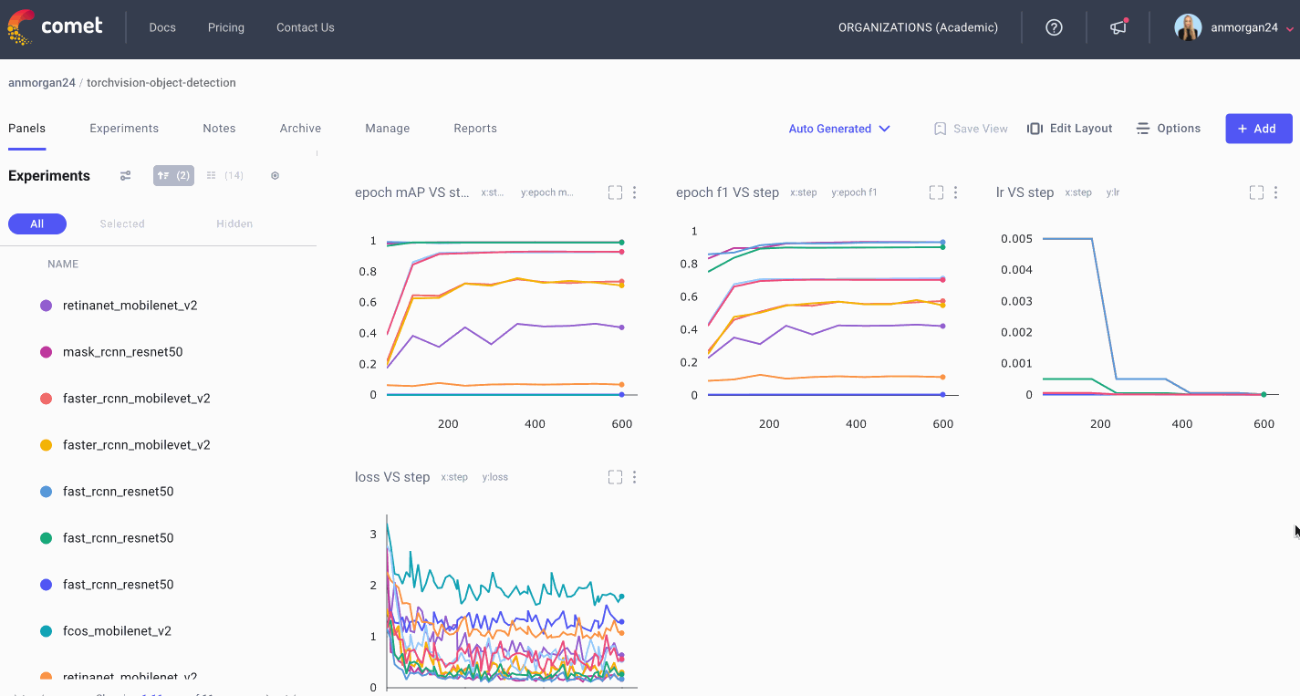
Multiple Dashboards
Now that we’ve built all of these panels, we need a way to keep them organized! For this, we build and save multiple dashboards, each of which we’ll use for a different purpose. We’ll keep the auto-generated dashboard that Comet built for us, and we’ll organize the rest of our panels into four more dashboards. We have a project overview dashboard that gives us a very basic overview of our project’s stats (parameters used, number of experiments run, and some of the best metrics achieved). We’ll put our image panel and data panel into a Debugging dashboard and we’ll store our plots and charts in a Metrics dashboard. Now we can easily navigate through all of our panels to find exactly what we’re looking for!
Accuracy Speed Tradeoff
At the beginning of this tutorial, we briefly explored machine learning’s accuracy-speed tradeoff. Models with higher precision and accuracy tend to consume more compute resources, and fast models tend to be be less accurate. Depending on your use case, your definition of the “best” model may vary. Circling back to this thought, we’ll compare four of our models in terms of their general speed and accuracy in order to understand which models work “best” for which scenarios.
We create a final dashboard called “Accuracy-Speed Tradeoff” and plot some basic evaluation and system metrics for four different models: Mask RCNN, Fast RCNN, RetinaNet, and FCOS. Remember that both RCNN models are two-stage object detection models, which are generally more computational expensive. RetinaNet and FCOS are both single-stage models.
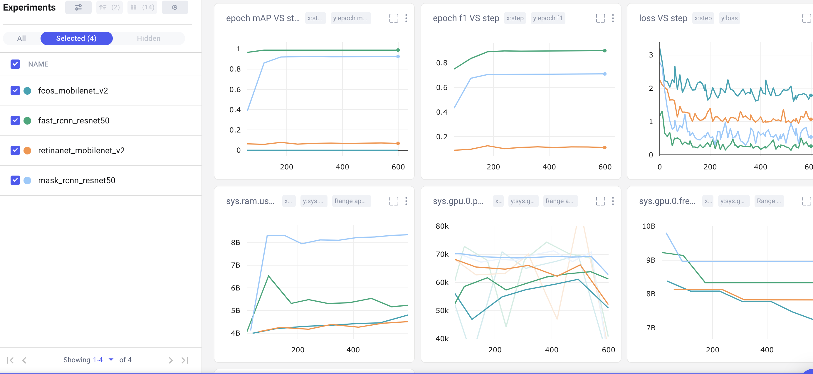
Choosing the Best Model
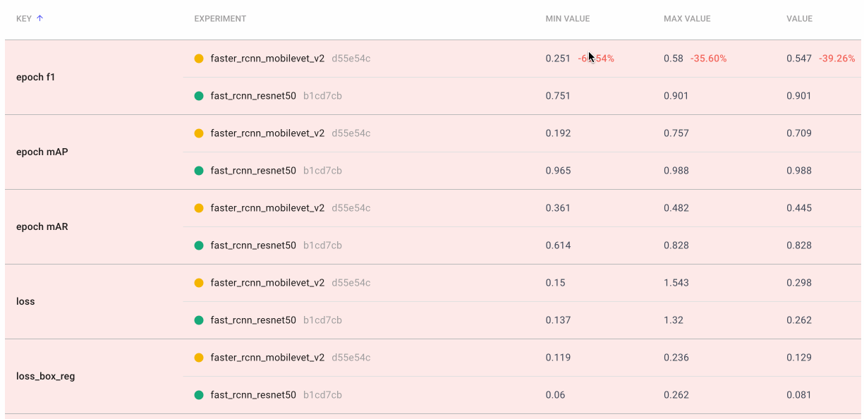
Both of our two-stage object detection models (in green and light blue above) far out-perform the single-stage models in mean average precision, epoch f1-score, and loss. Shifting to the bottom row of charts, however, we can see that they are also much more computationally-expensive. It may come as no surprise that Mask RCNN is the slowest model of all, because it’s based on Fast RCNN, but with additional outputs (masks).
For a general purpose object detection model, we might conclude that Fast RCNN performs the best with bounding box prediction. It has the highest mAP and f1, the lowest loss, and consumes far less memory than Mask RCNN. But the “best” model is subjective and entirely dependent on your use case! If we were looking to deploy our model to a mobile device, Fast RCNN’s memory requirements might disqualify it from our consideration.
Conclusion
Comparing and logging object detection models can be a tedious and overwhelming task, but when you have an experiment tracking tool like Comet, you can focus your attention where it really matters. Comet is a powerful tool for tracking your models, datasets, and metrics to keep your experiments organized, reproducible, and explainable.
Try out the code in this tutorial in this Colab and apply it to a dataset of your own! You can view the public project here or, to get started with your own project, create an account here for free!
