A Deep Dive into TFRecords and Protobufs
Learn how to optimize your deep learning pipelines using TFRecords and Google’s Protobufs (protocol buffers) in this end-to-end tutorial.
Introduction
When it comes to practicing deep learning at home vs. industry, there’s a huge disconnect. Every course, tutorial, and YouTube video presents you with a nicely prepared dataset to feed any DL algorithm for any DL framework. TensorFlow itself comes with the Dataset API that allows you to simply download and train data with just a couple of lines of code. However, when it comes to real life production work at a company, nowhere on this earth will someone just hand you a pristine dataset ready for consumption. Considerations must be given to things like:
- File format: Are flat files sufficient, should the data be serialized, etc.
- File Structure: Should there be a pattern to the directories for separation of training examples vs labels, some hybrid data structure, etc.
- Data location: Can the data be batch fetched from the cloud or does it need to exist locally
- Data Processing: Is there another system responsible for collecting and processing the data? And is that system in a completely different framework or programming language: If so, how much effort does it take to go from that system to a deep learning framework-ready system?
- CPU/GPU: Are you limited to only CPU processing (hopefully not) or is there GPU access
Although not as sexy as model building, these items are important since time is money. Slow input pipelines means slow training time, which has a few consequences. The longer it takes a model to train, the longer engineers must wait between iterations for tweaking and updating. This ties up said engineers from working on other value propositions. If a company is utilizing cloud resources, this means large bills for resource utilization. Also, the longer a model is in development, that’s time lost it could have been in production generating value.
TFRecords
So today, we are going to explore how we can optimize our deep learning pipelines using TensorFlow’s TFRecords. I’ve seen a few blogs on this topic, and all of them fail to adequately describe what TFRecords are. They mostly regurgitate example from docs, which themselves are quite lacking. So today, I’m going to to teach you everything you wanted (and didn’t want) to know about TFRecords.
The TFRecord format is a protobuf-backed format for storing a sequence of binary records. Protobufs are a cross-platform, cross-language library for efficient serialization of structured data. Protocol messages are defined by .proto files, these are often the easiest way to understand a message type.
Protobufs?
So what is a protobuf (aka protocol buffer)? To answer that question, I’m going to mix some technical jargon with some actual examples that explains the jargon.
Protobufs are a language-agnostic, platform-neutral, and extensible mechanism for serializing structured data. They were developed by Google and released as an open-source project. Protocol Buffers are widely used for efficient and reliable data exchange between different systems, especially in scenarios where performance, compactness, and language interoperability are important.
Now all of that may or may not mean anything to you, but let’s explain it by stepping through all the pros of using protobufs. We are going to touch on:
- Language Interoperability
- Forward & Backward Compatibility
- Efficiency
- Schema Validation
1. Language Interoperability:
Protocol Buffers provide support for generating code in multiple programming languages, enabling different systems written in different languages to communicate seamlessly by sharing a common data structure.
Let’s say I want to create a system that collects social media posts from people so that I can train models with the data. The backend of the site is written in Golang, the web scraper might be written in C++, the data cleaning and preparation might be written in Python. By using protobufs, we can define the schema once, and compile for all the aforementioned languages. This empowers a “write once — use everywhere” type of system which drastically reduces engineering time.
Conversely, if we were to pass around our data as say, JSON or XML, we would have to individually write wrapper classes or objects for each language to consume that data. That opens the doors for a lot of bugs, mistakes and maintenance. For any update to the data schema, you must update a bunch of code across a bunch of different frameworks.
Implementing Protobufs
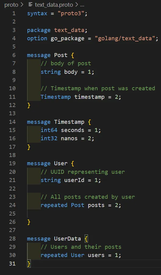
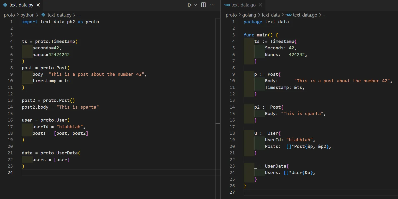
We start off defining our protobufs by creating a file called “text_data.proto”. We then define the attributes of a “Post” which would be comprised of a body of text and when it was written.
Notice that we are defining the data types for each attribute. This is because all code generated by the proto file will be strong, statically typed objects. Yes, even in python (we will see this later). Next, a post would belong to a user. That user may have 0 or more posts. So let’s define that.
We define 0 or more posts by using the “repeated” keyword. This signals to the protobuf compiler, at compile time, that the generated object should be an array of some sort that holds objects of type “Post” and nothing else. Finally we just need a way to collect all the users and their posts in a single parent object.
Each of these messages defines individual objects that will be created for any language we compile for. The overall proto file should look like this:
In order to compile, you need to install the protoc command line tool. I won’t go into super details on this part because it’s not overly important to this post. This is just a quick crash course on protobufs and what they are. You won’t actually need to do this when it comes to TFRecords and training models. This just sets the basis for what comes later.
Compiling for Golang
Again, don’t worry too much about this since you don’t really need to do this, but this just signals to the compiler to generate Golang code using the define protobufs in the proto file. Once we run this, it will generate a file called “text_data.pb.go”.
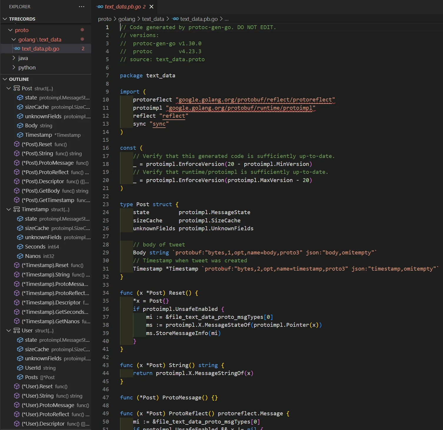
What this file is, is the Golang version of what we defined. It uses Golang native data types and structures. Golang doesn’t have classes. Instead it uses C-style structs. And you can see that there is a Post struct, representing the message “Post” we created. In the outline section on the left, you can see it created Structs for all the messages we defined, and a bunch of other methods and goodies. Some of these goodies allows us to represent our object as a string to print to console if we so choose. It also gives us the capabilities to convert our protobufs to and from JSON objects.
Compiling for Python
When compiling for Python, you get something different. You don’t get actual Class implementations of our protobufs, you get a Metaclass.
“Metaclasses are deeper magic than 99% of users should ever worry about. If you wonder whether you need them, you don’t (the people who actually need them know with certainty that they need them, and don’t need an explanation about why).”
— Tim Peters
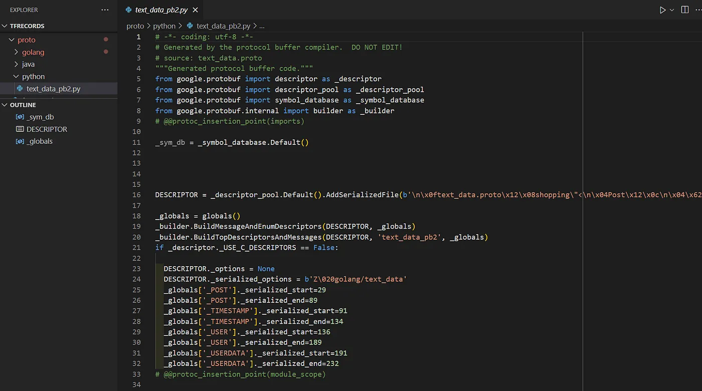
You can see on line 16 in the Python generated code image above that there is a DESCRIPTOR variable that is being injected with a serialized definition of our proto. Although cut off in the image, that serialized string is extremely long. This description is used by the Meta class to ensure that any instance of our protobufs in Python code strictly adhere to the definition in the proto file. We will circle back and talk about this more.
When we are ready to use our newly compiled protos, we just import them and use them as if they were a native object for the programming language we are working with. The best way to think of protobufs while using them in your codebase is as “value classes”.
For those who don’t come from CS or SWE backgrounds, a “value class” typically refers to a specific type of class or data structure that represents a single value or entity. A value class encapsulates a value and provides operations or methods related to that value, but it does not have identity or mutability. Tangential examples would be Autovalue in Java, Data Class in Kotlin, and the Data Class decorator in Python.
2. Forward and Backward Compatibility:
Protocol Buffers support versioning and evolution of data structures. You can add new fields to a message without breaking existing code that was built with the previous version of the message. This allows for easier maintenance and updates in distributed systems.
This one is very simple in explanation. If we ever want to change or improve any of our protos we can simply add a new field. If this field is meant to replace an old field, all we have to do is mark that old field as deprecated. Any new code using our protos will be flagged to not use the deprecated field. Any old code that isn’t aware of the new field will still work as intended because we never actually removed the old field.
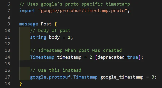
This is far better than JSON or XML. If you are expecting JSON/XML version ‘X’ but you get version ‘Y’, your code more than likely won’t work. Or It will fail to parse properly because there’s new fields your code isn’t aware of. Or worse, there’s fields that have been removed that your code is expecting to be there. Here, we don’t have that problem. Backwards compatibility will always exists as long as you don’t delete the field from the proto message. There’s also no penalty for not using a field either.
3. Efficiency:
Protocol Buffers are highly efficient in terms of both space and processing time. The serialized data is usually smaller than equivalent XML or JSON representations, resulting in reduced storage and transmission costs. Additionally, the encoding and decoding operations are faster, making it suitable for high-performance systems.
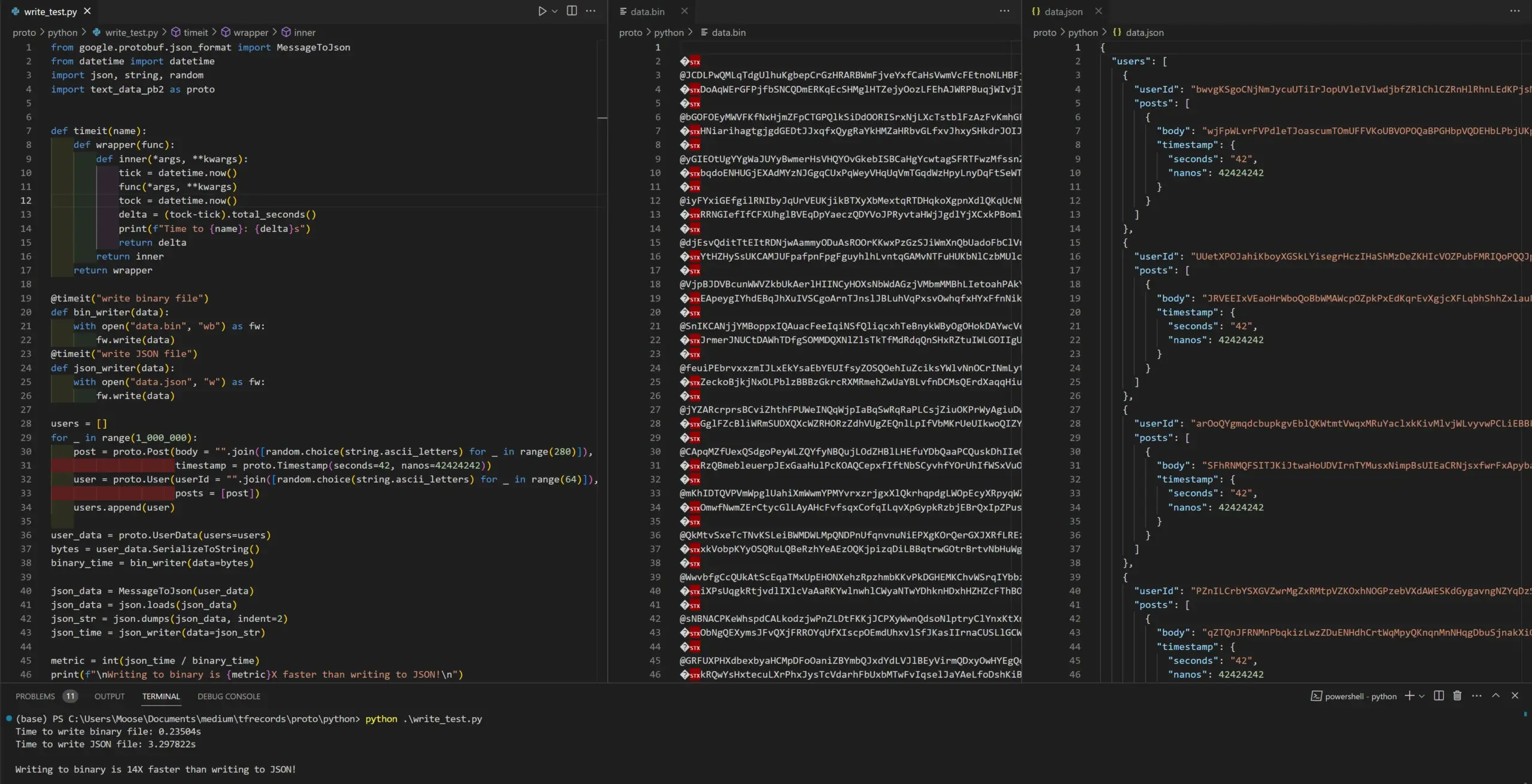
As a demonstration, we will create 1 Million users, each of whom have written a social media message with the maximum character length of 280 characters. We will then write the data both in a serialized binary format as well as JSON format from the proto. As I said earlier, protos afford you the ability to transition back and forth between JSON as long as you adhere to the strict schema. We will then time the write operation, as well as inspect the overall file size written to disk.
4. Schema Validation:
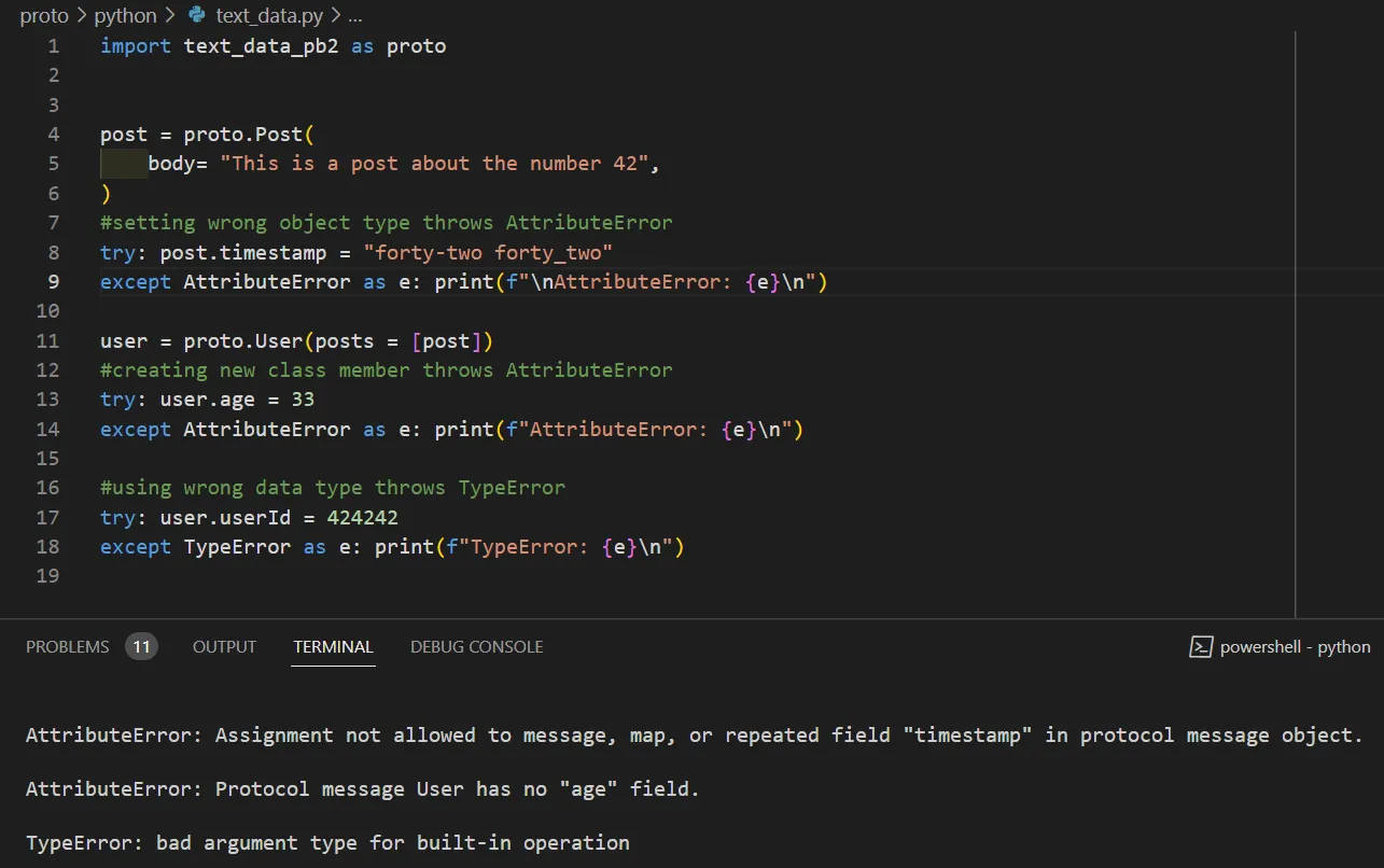
The defined message structures in Protocol Buffers act as a schema that can be used to validate the data being exchanged. It ensures that the received data adheres to the expected structure and type constraints. The reason for Python Metaclasses (as shown earlier) is because protobufs inherently provide type safety — meaning they have defined types that must be obeyed. They are immutable, and the structure of the class must not and can not ever change. I.e. what we defined in the proto file and generated by protoc should be exactly how the class is…..always.
No code at runtime is allowed to change the structure of the class, only the data it contains. Python on the other hand, is a dynamic “duck-typing” language that has no true concept of static types. Nor does it have any native access modifiers that make members private or protected. The below examples are problems with Python with respect to protobufs.
Thus, the metaclass ensures we follow the exact structure and types as defined in the proto file. This type safety is what enables the platform agnostic nature of protobufs. We can’t alter or add anything to a protobuf at runtime that wouldn’t be understood by the same protobuf running on a different platform.
Enforcing this in static typed languages such as Java, C++, & Go is pretty straightforward. If you defined a variable as some type, it can only ever be that type. These languages also come with access modifiers so that you can make fields private and non accessible from outside the class. This way, as you pass the protos from system to system that utilize different platforms, they still know how to handle the data since we know it adheres to the strict schema of the proto.
Protobuf Conclusion
Overall, Protocol Buffers are a powerful and flexible tool for data serialization and interchange. They are commonly used in various domains, including distributed systems, APIs, communication protocols, and data storage formats. These are only a few benefits of using them since we never even touched on data transmission across networks. Which, as a quick aside to this point — protobufs are the backbone for:

Which if you are unfamiliar with gRPC, I highly suggest you checkout the docs. In short, it’s a better framework than REST services. It supports HTTP/2 and enables full duplex communication. This means faster network transfers and less network requests, all powered by protobufs! Something to think about as you’re constantly requesting the next batch of data from remote storage to train your model.
Protobufs for TFRecords
So why the heck did I just spend all that time covering protobufs. Well, that’s because at the heart of TensorFlow’s TFRecords, are protobufs. You can view the actual proto file here. But we are going to step our way through this file, message by message.
The comments at the top of the proto file already provide an example data structure using movie data as the example data. We will just use the same information to make our way through the explanation. So go ahead and open up that file now and take a look as we go through this.
The most basic component of a TFRecord (and by extension, the protobufs that make up TFRecords) is data that consists of one of three types
- bytes — Would be used for text, audio, or video based features/inputs.
- float — Would be used for features/inputs with floating point precision e.g. 3.14
- int64 — Would be used for features/inputs with simple integer values e.g. 100
The basics
Representing this in the TFRecord, there are three proto messages defined.
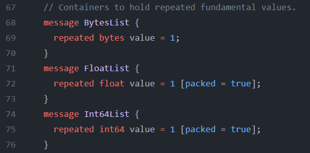
The initialization and utilization for any of them would require 0 or more entries of data consisting of the specified data type. This is due to the “repeated” keyword. This signals to the proto compiler that this field is not a single value, but it is an array of values of the defined data type.
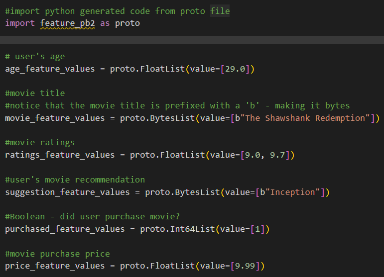
I’ve taken the proto file from their git repo and have compiled it. I’m using the generated code in the examples that follow.
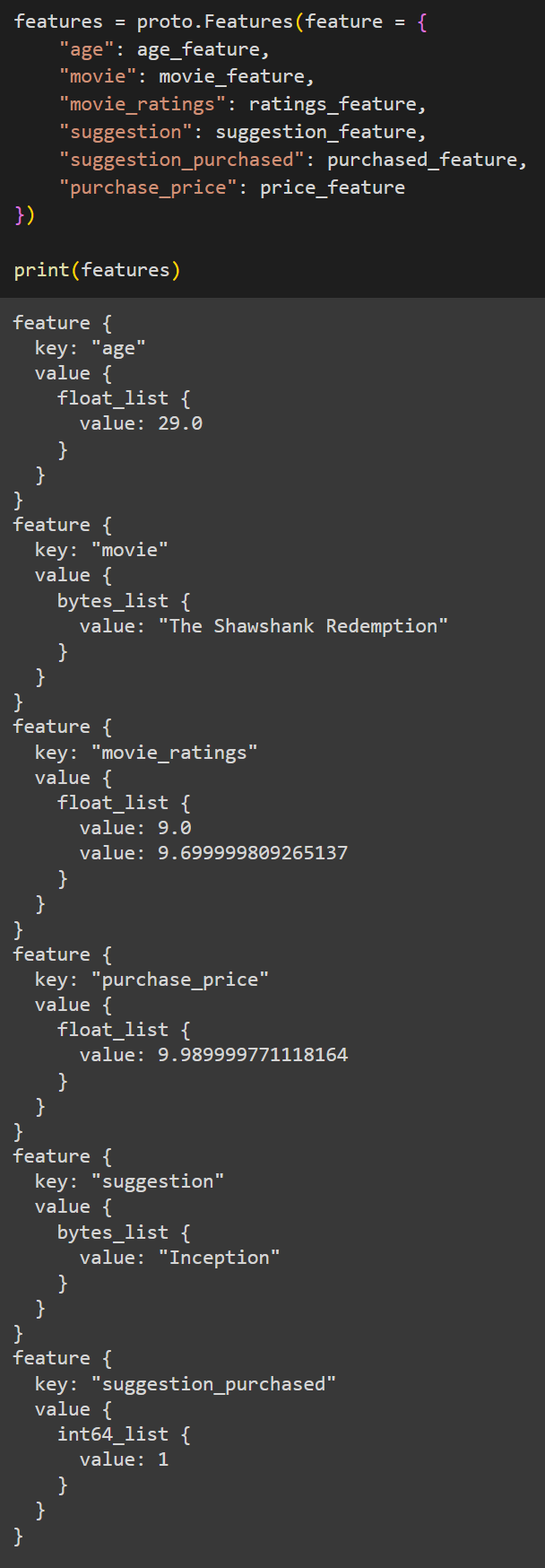
Since this is just the raw values with no labels, we need a way to itemize the data. Obviously this would be necessary for data understanding as well as feature engineering. To do this, we first create a “Feature” proto.
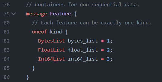
The “oneof” keyword signals to a user that this proto will be a feature containing one and only one of the base proto types. When compiling a proto with protoc that contains a “oneof” member, it also generates extra API for type-checking capabilities. This makes it so a user and/or code can inspect the proto and determine which “kind” it contains. And of course it also enforces that an instance of the feature proto can, and will, have a single type. Otherwise a run-time or compile-time error will be thrown depending on the programming language being used. You can read more about the “oneof” keyword here
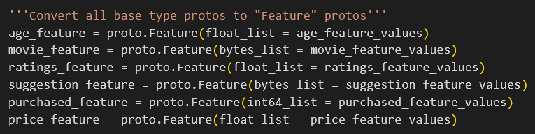
But wait, why did I create the individual protos of ByteList, FloatList, and Int64List just to wrap them in yet another proto? Well this is mostly a design choice. And whether you feel like it’s a good one or not, simply boils down to philosophical differences. But the next part might shed some light on this design choice.
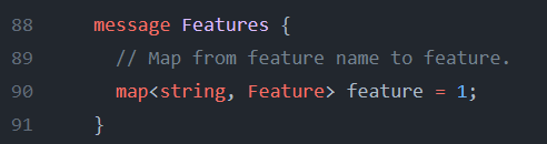
Feature proto map
After we have created our Feature protos, we still need a way to assign a label to them. And we do this by aggregating all of our newly created features in a feature map proto called “Features” (unique naming, I know). In this proto map, each feature we have created is indexed by a string key. If you’ve only been programming in Python land your whole life, and have no clue what I mean when I say map, you can think of it as no different than a Python dictionary. It’s a key-value data structure.
Because our raw data is contained as either BytesList, FloatList, or Int64List and wrapped in a “oneof” Feature proto, that simplifies the map (and thus justifies the design choice). If we weren’t wrapping the base protos in the Feature proto, then we would have to create an individual map member for all the base types. For example, “Features” would have to become:
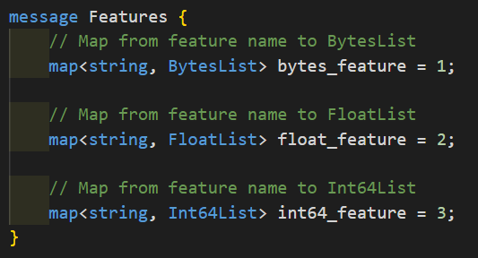
Again, if you’ve only ever programmed in Python, or something of the sort, this might seem strange to you. But unlike Python, which is dynamic and doesn’t enforce declared data types, protobufs are strongly type. You can’t create arrays or maps and insert mixed data types into them. Hence we would have to make our Features proto like above. But this would be more cumbersome to deal with in practice. Instead of having a single map containing all of our data, we would now have to inspect 3 separate maps for the possibility of any data.
TFRecords in Tensorflow
If you’ve ever looked at the documentation in TensorFlow for utilizing TFRecords, of if you’ve ever just used them in practice, you may realize that the API docs don’t actually import any generated protobuf files, nor does it mention anything of protobufs apart from the fact that TFRecords are backed by protos. This is because the TensorFlow API has its own wrappers and abstractions around the protos. Quite conveniently however, the TensorFlow API almost matches exactly what we did with the raw protobufs 1:1.
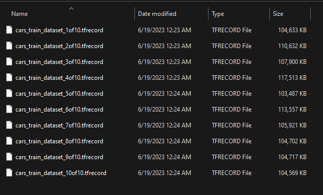
Writing TFRecord Files
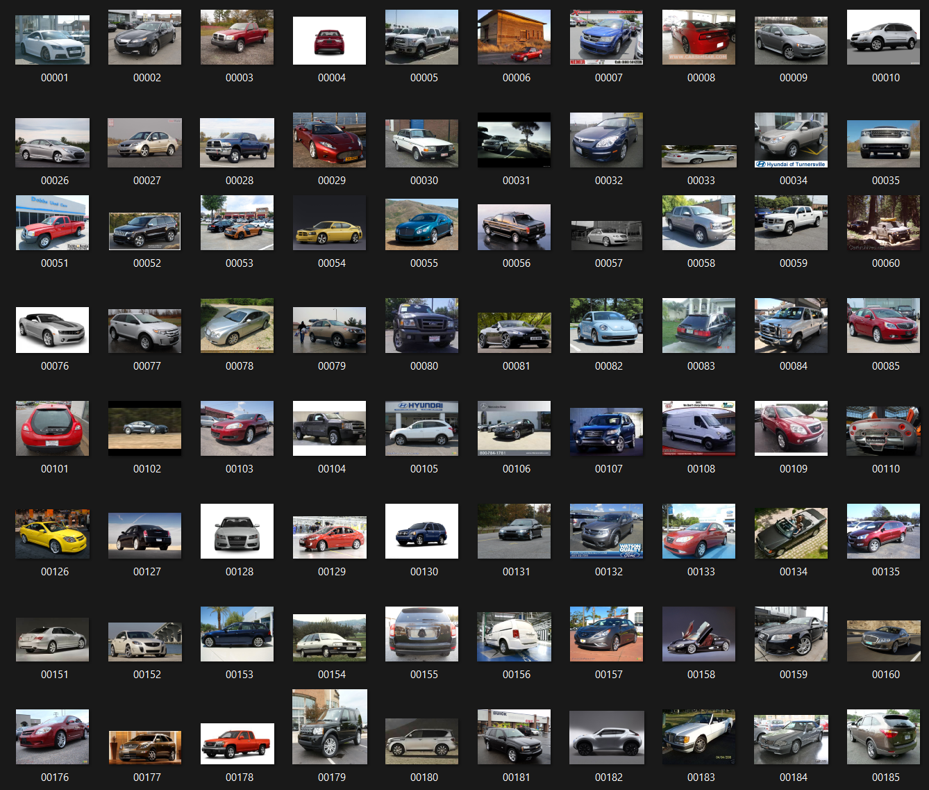
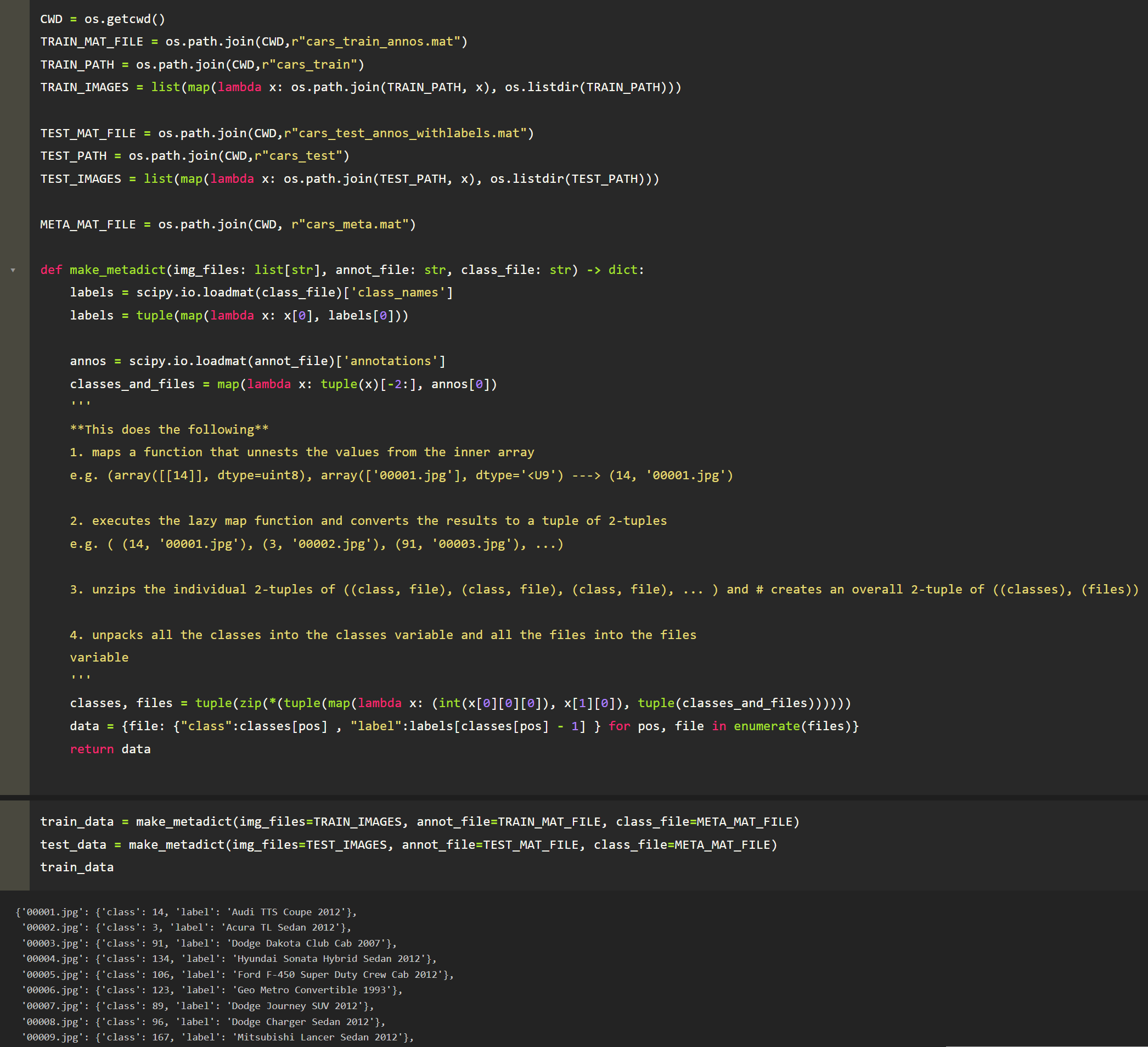
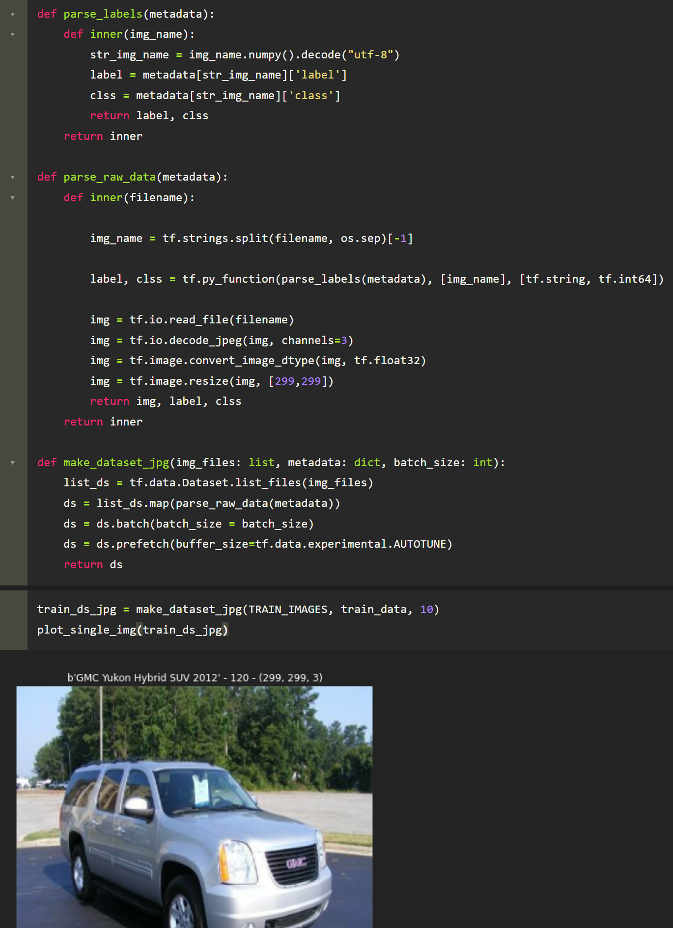
To demonstrate creating TFRecords using the TensorFlow API, I’m going to use the Stanford Cars Dataset. This is a great example dataset to use in this demonstration since all the training images are contained in a single folder and their actual labels and names are in a separate “.mat” file. We can use this opportunity to not only convert these images from JPG to TFRecords, but when converting them, we can even write them with their appropriate label and any other metadata we wish to store with the image itself.
Before we start though, let’s do some setup steps. Because the names and labels for each car are in a separate file, lets create a dictionary where the keys are the image names — e.g. “00151.jpg” — and the values are another dictionary containing the car name and the class label of the car for classification. This label is represented as an integer in the data. Some example entries of the dictionary would be
Since this isn’t an article on data cleaning/preparation, for this initial step, I’m just going to show my code with comments. I’m not going to explain it.
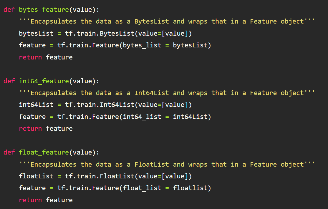
To better organize the training data, each individual image will be converted from its JPEG form to a TensorFlow “Features” object. Remember that the “Features” proto is a map of string to feature. The same holds true for the TensorFlow “Features” object. Thus for a single image, it will be represented in the following manner:
Defining our helper functions
Following the same pattern that we did above when we were using the actual protobufs, we first need to convert each of these features into either a TensorFlow BytesList, FloatList, or Int64List object. We then need to wrap that newly created Bytes, Float, or Int64 list, in a TensorFlow “Feature” object(not “Features” — again, unique naming, I know). We will create helper functions to do so. This part is where you typically see most tutorials on TFRecords start!!!!
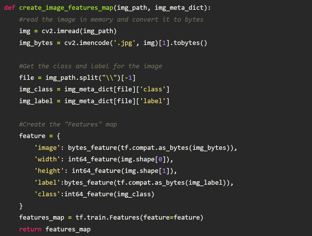
Next, We will create a helper function that will
- Read an image into memory
- Extract its name and label from the dictionary in the preprocessing step
- Convert the image to bytes
- Convert all features into either a bytes, int64, or float feature
- Create the final “Features” map object.
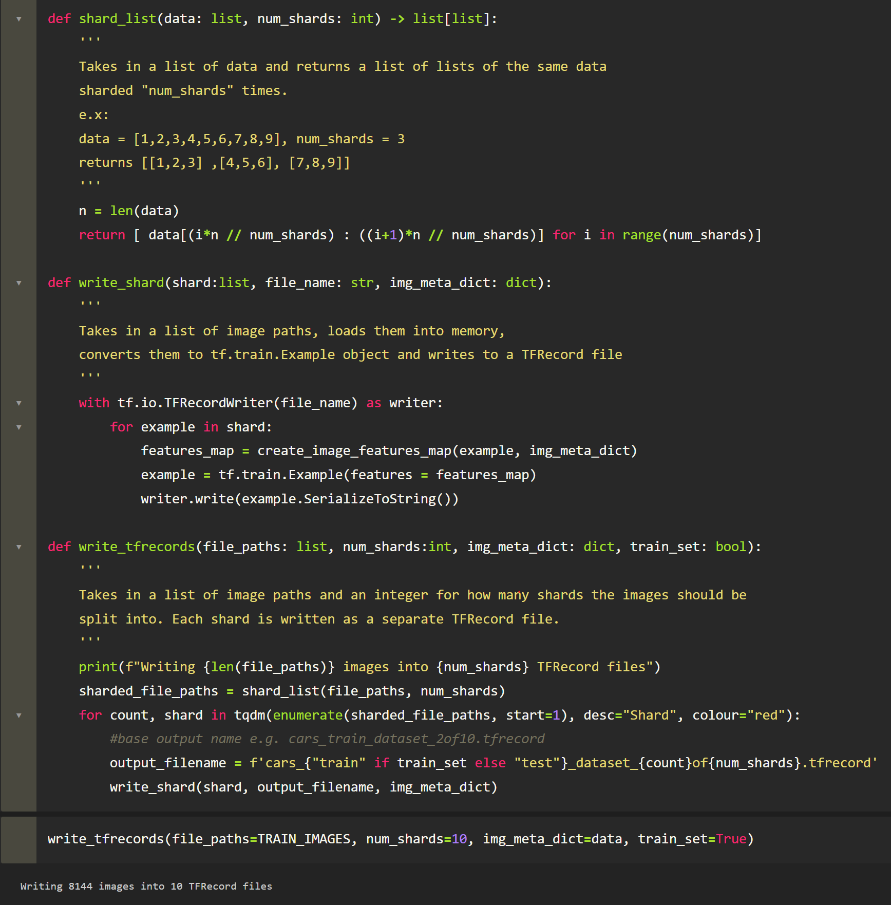
With our helper functions done, all we need to do now is to:
- Get a list of all the images in the train directory (their paths)
2. Shard them into a certain amount — e.g. a list of 50 pictures sharded into 5 sets would result in 5 lists of 10 images
3. Write each shard as a separate TFRecord file.
Last thing of note — before we write the data as TFRecord, we will wrap the features map object in one last object, the tf.train.Example object. Once in that form, we can write to disk. There is no requirement to use tf.train.Example in TFRecord files. tf.train.Example is just a method of serializing dictionaries to byte-strings.
Reading TFRecords
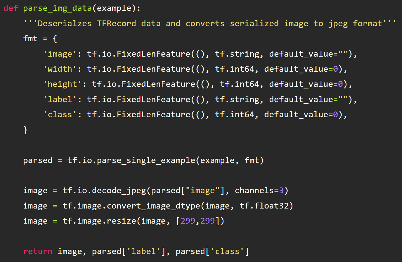
Reading the TFRecords and preparing them for model training is straightforward and doesn’t deviate very much from all the examples in the tf.Dataset docs. We will write a couple of helper functions. The first helper function will allow us to parse a TFRecord file that is loaded into memory. Since the data is serialized, we need a way to deserialize it. We do that by first defining the expected schema of the data in a dictionary format so the parser knows what to expect.
You can see that this follows the same dictionary format we created when first wrote the TFRecord files. This informs the parser that it should expect to be able to deserialize the data into the 5 feature fields of image, width, height, label, and class. It also informs the parser of the expected data types as well as the default value if the data is missing for that particular feature.
Decoding the binary file
You might be asking yourself why you need to yet again define the structure of the data if you already did so when writing the TFRecords. Well this is because the data is serialized in one long string of information. Without giving the parser the expected structure of that information, it doesn’t know how to interpret it. Think of it this way, if I just gave you the binary of:
01000001
In pure binary, this is just the number 65. However I might have intended for you to parse it as ASCII, and in that case this is actually the letter ‘A’. Without the extra information, there’s ambiguity as far as what the data could actually mean.
Next we need to convert the serialized image back into matrix form. I’m also going to take this opportunity to resize the image since I’m going to use a pre-trained model that expects image input to be (299,299,3).
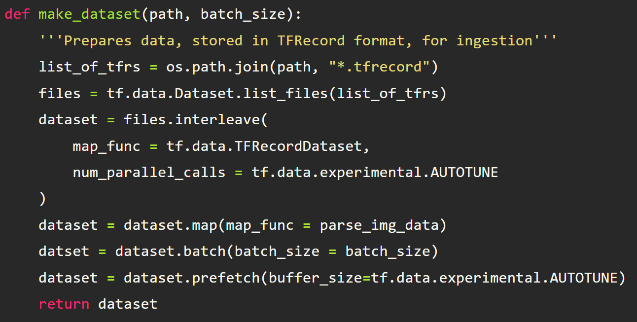
Configuring out input pipeline
For the next step we will use the TensorFlow Dataset API and configure our input pipeline. To do this, we need to tell TensorFlow where the files are and how to load them.
The actual loading of the TFRecords is handled by the mapping function TFRecordDataset. What the interleave method does is it spawns as many threads as you specify, or how many it thinks is optimal if you use the AUTOTUNE parameter. Each thread with load and process its own part of the data concurrently. So instead of processing a single file one at a time, many can be processed at once. As each thread finishes processing a portion of its data, TensorFlow will “interleave” the processed data from various threads to make a batch of processed data. Hence instead of loading and processing a single file and making all the data from that file a part of a batch, it will gather data randomly from the various threads and create a batch.
After the data is loaded, we need to apply our parsing function we created above as well as other pipeline parameters such as batch size and prefetching.
The prefetch method basically tells the CPU to prepare the next batch of data and have it ready to go while the GPU is working. That way, once the GPU is done with its current batch, there’s minimal idle time while it waits for the CPU to prepare the next batch.
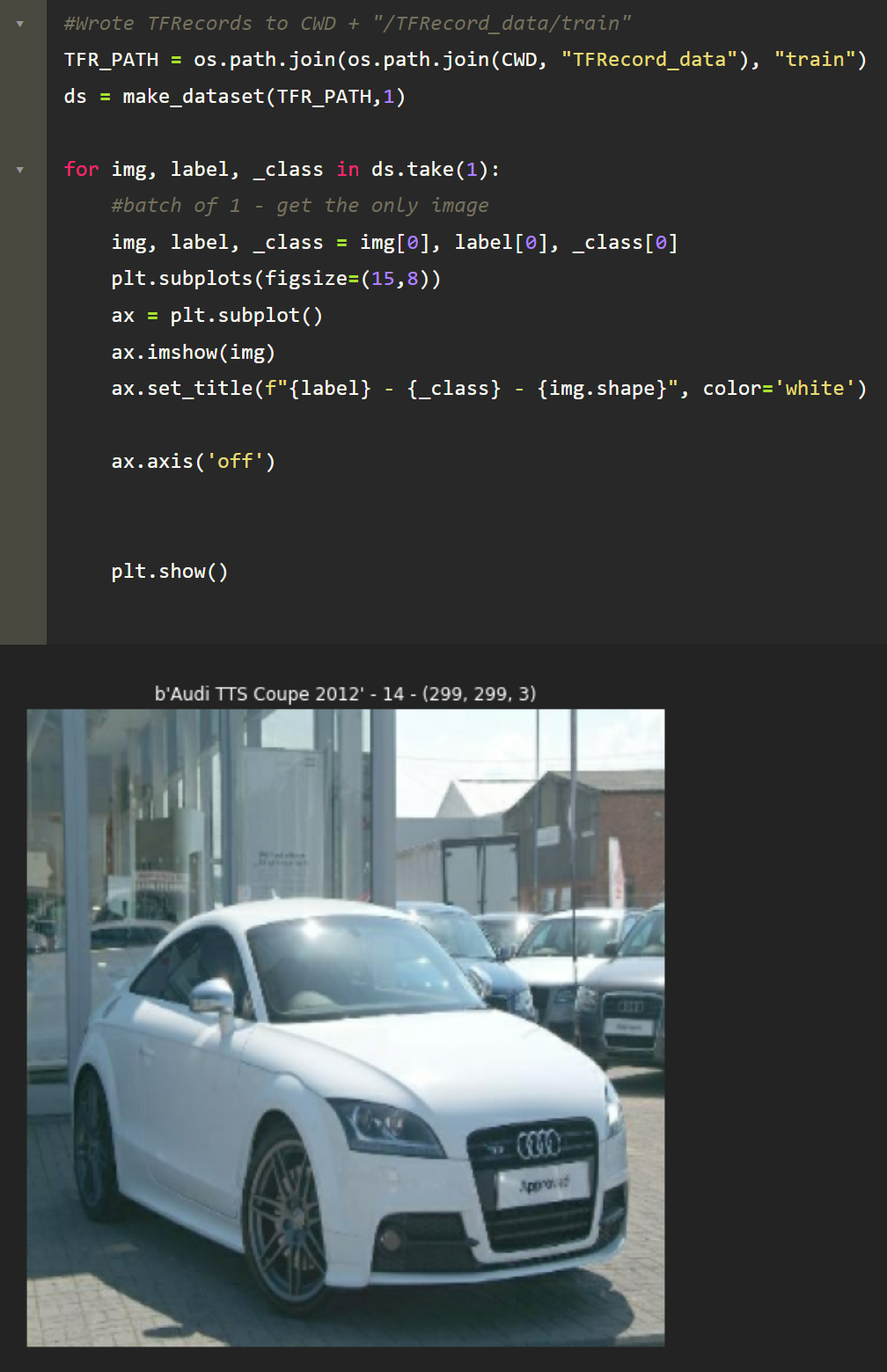
And that’s it for reading the data. We can now test it out and plot an image as well as inspect the image size transformation.
Training with TFRecords vs Raw Input
Most deep learning tutorials, both PyTorch and TensorFlow, typically show you how to prepare your data for model training by using simple DataGenerators which read the raw data. With this method, you are (lazily) reading the data from disk in its raw form. In our case, a DataGenerator with batch size of 10 would have to read 10 separate JPG files into memory prior to any other preprocessing in the pipeline. To compare how (in)efficient this is compared to TFRecords, let’s create our own DataGenerator that still uses the same pipeline as our TFRecords. The steps for this will be
- Create a helper function that gets the class and label from the meta-dictionaries we made in the preprocessing step.
- Create a helper function that reads the image into memory and bundles it with it label and class as retrieved in the previous in the helper function.
- Returns the data generator with applied pipeline settings of “batch size” and “prefetching”
Monitoring Training
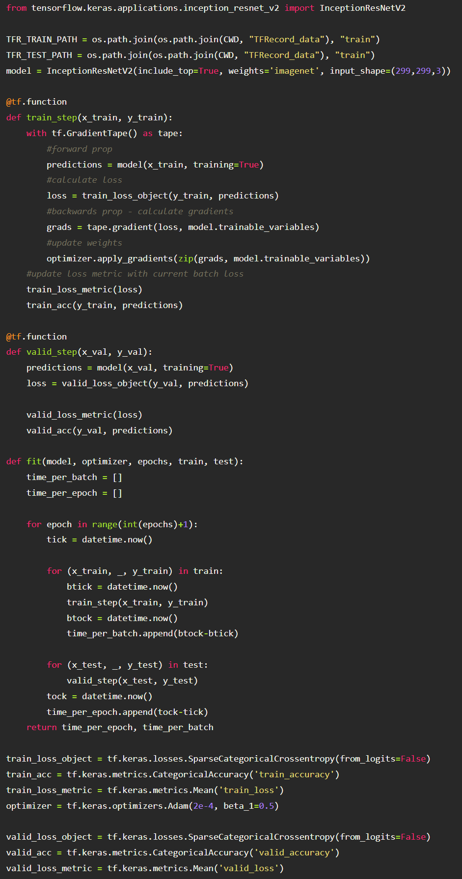
We don’t care so much about the actual model for our testing. So we will just use transfer learning and load InceptionResNetV2 model. What we do care about is
- CPU Utilization — When is it active and how long is it active for
- Memory Utilization — How much memory is being used for processing of the data prior to loading to the GPU
- GPU Utilization — How much idle time does the GPU experience while it is waiting for the CPU to prepare the next batch
- Time to train between each batch
- Time to train between each epoch
To monitor the utilization, we will do two separate things that ultimately achieve the same goal. The first one requires more work by you, the second handles everything for you after minimal setup using Comet’s online dashboard.
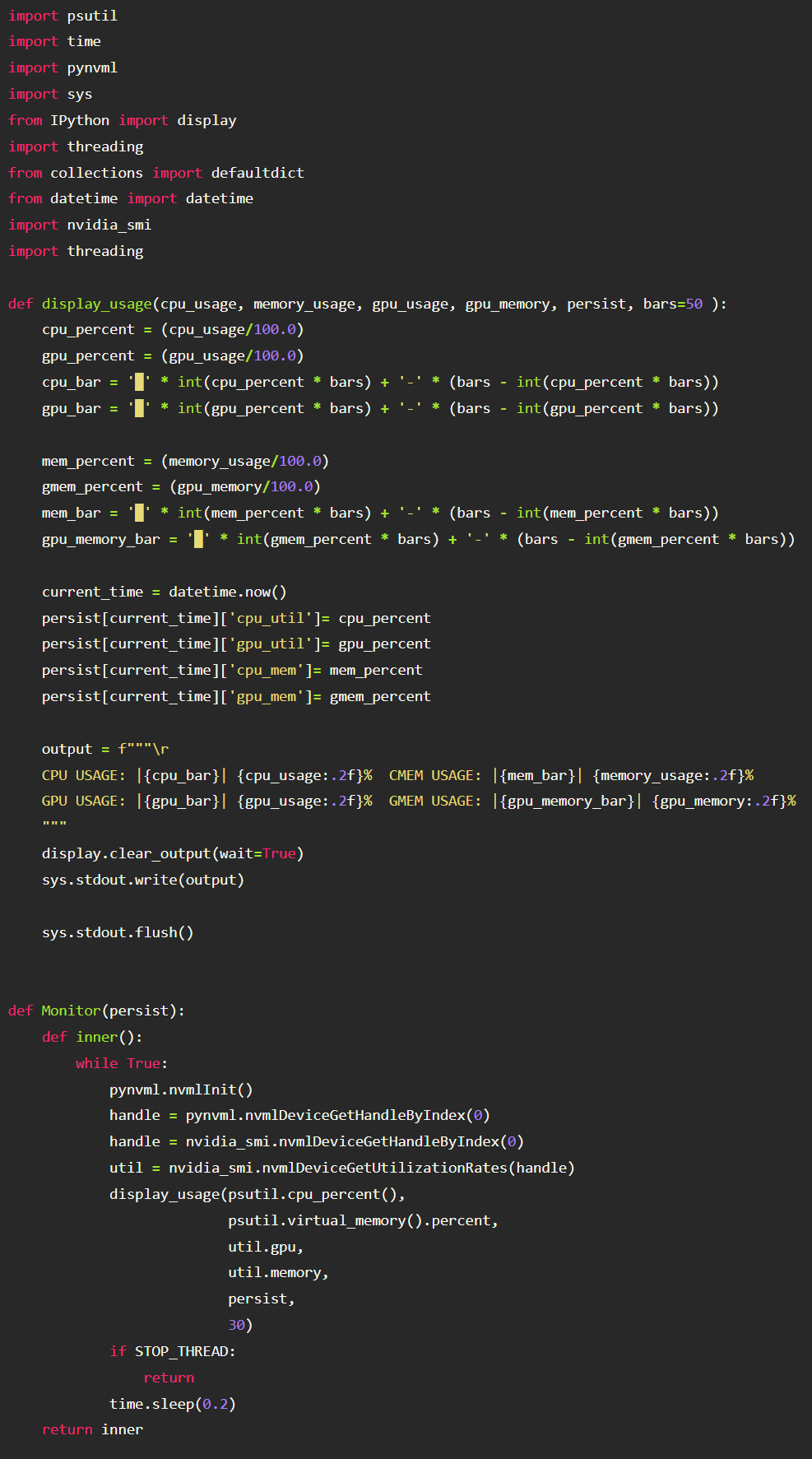
Manually logging system resources
1. We will spawn a separate thread (so it’s not blocking our model training) and sample utilization metrics 5x a second. Below is the code for this operations. Again since this isn’t an article on logging system resources, I leave it to the reader to figure out the code.
Logging with Comet
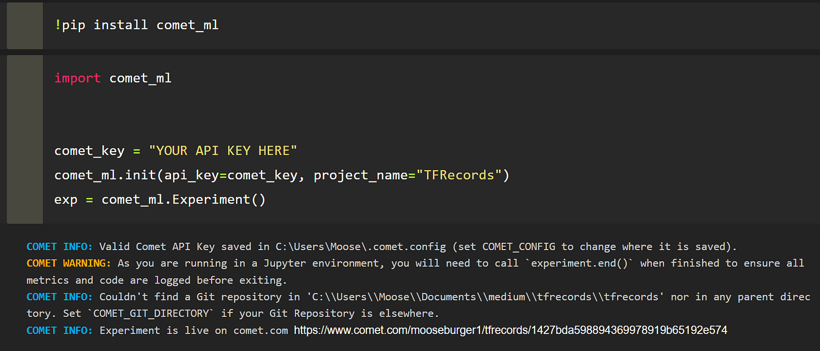
2. We will use Comet.ml to log our metrics to a web based dashboard. We will do this so we can chart in real-time the performance of model training with respect to both datasets as it’s training. If you’re not familiar with comet, you can just head over to Comet.ml and sign up for free. You will need your API key. After you create your account, click your profile pic in the top right corner, then go to Account settings, On the left navigation panel, you will see API Keys . It is here where you can find your key.
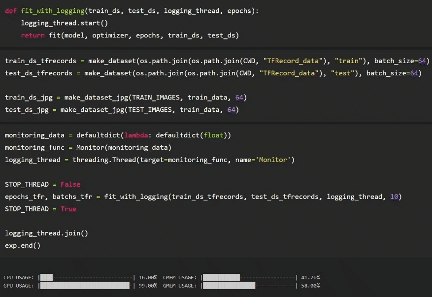
To log the time between batches and epoch, we will simply have the data written to a list during training. We could also log the batch and epoch information to Comet as well. However I prefer to collect the data locally so that I can do some extra analysis and plotting after the fact for this blog post. The entire training loop is the following:
Parameters
System parameters:
- RTX 3090 24GB Ram
- Ryzen 5950x 16 Core 32 Thread CPU
- 64GB DDR4 Ram
- ASUS Crosshair III Formula X570 Motherboard
- 2 TB Samsung EVO SSD
Test parameters
- batch size = 64
- epochs = 10
- prefetching = True
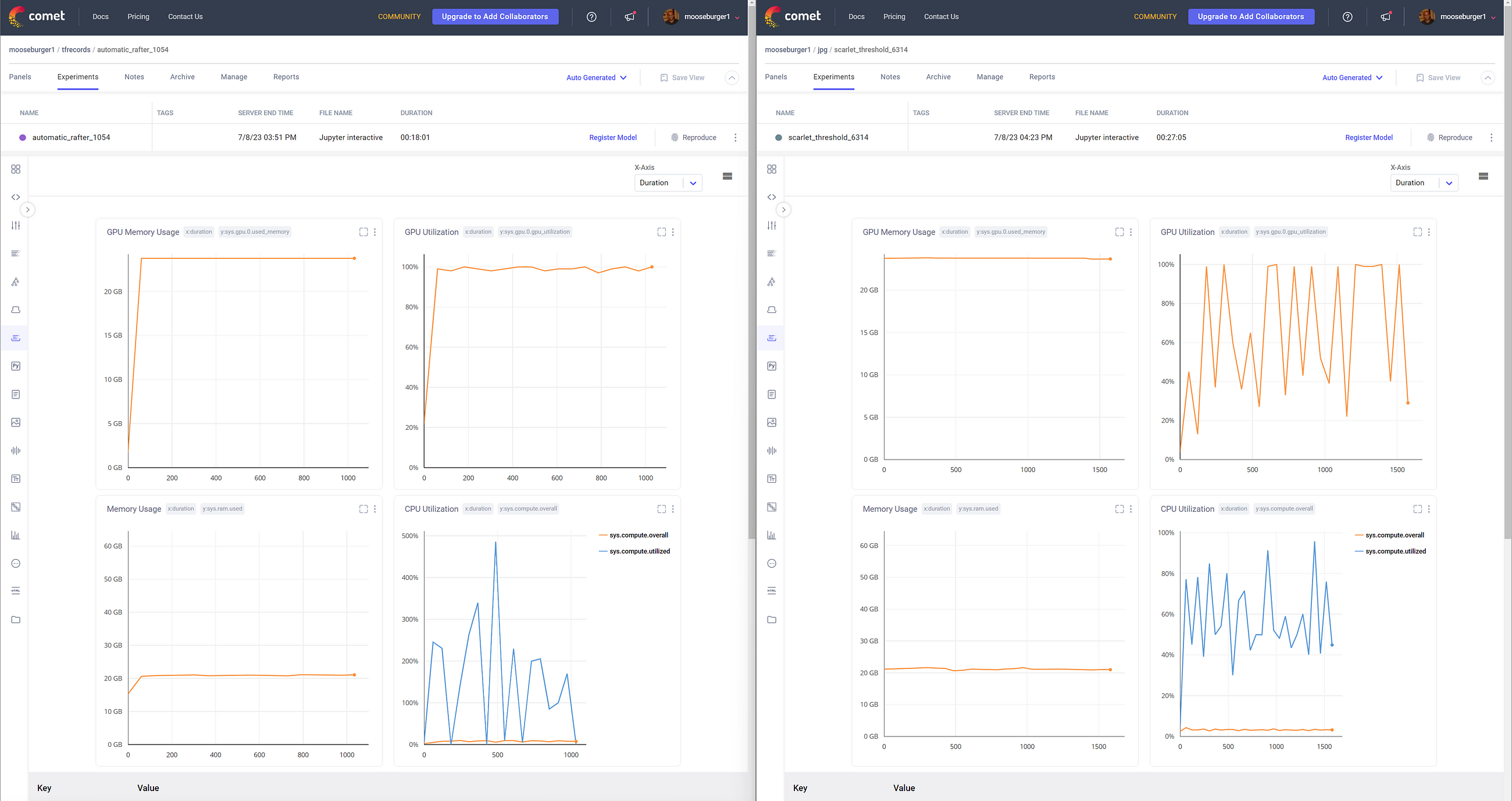
Below shows the setup, testing and logging using the TFRecords first. As the model is training, Comet is logging system resources for us after we have setup the experiment as seen above. Notice that we call exp.end() after the model is done training. This will signal to Comet to stop logging. Also, our custom logging function is recording system resource utilization on a separate thread locally. It is recording that data to the “monitoring_data” dictionary we passed into the “monitoring_func”.
Results
While monitoring the metrics during training on Comet (image above), it was already clear how much more effective TFRecords were vs raw JPG on disk. The dashboard shows that the GPU was utilized almost 100% of the entire training loop. Conversely, the JPGs induced a lot of idle time. In the dashboard above, we can see that TFRecords took 18 minutes to train for 10 epochs, where JPG took almost >9mins longer, at 27 minutes to train. The Comet data was aggregated and uploaded at 1-minute intervals.
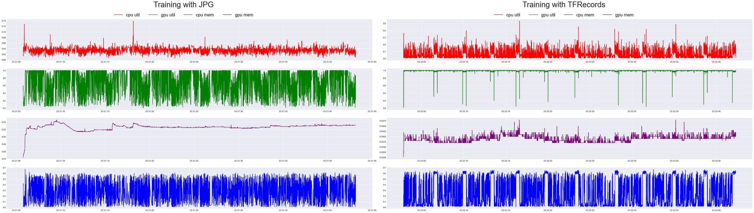
Looking at the data logged locally at a higher resolution (5x a second) — when training with the original JPGs, there’s a lot of “dead time” on the GPU while it’s waiting on the CPU to read each image, process it, and load it. Compared to the raw results of the training session with TFRecords, the GPU stayed busy almost the whole time as we saw in real-time on Comet.
Note:
As an FYI — When reading the x-axis, it is plotting a python DateTime as the value, so the first number on the axis is the date, not the time. Hence the value of 22:21:10 actually means day=22nd, hour=21, min=10. It also looks as if the CPU was never quite as busy than when it was training with the TFRecords. It’s almost as if it was working double time to ensure it was keeping up with the demand of the GPU. Which is why the GPU was so busy compared to just the raw JPG files. Let’s apply a Gaussian filter on the time-series and see if the smoothed curves reveal any further trends.
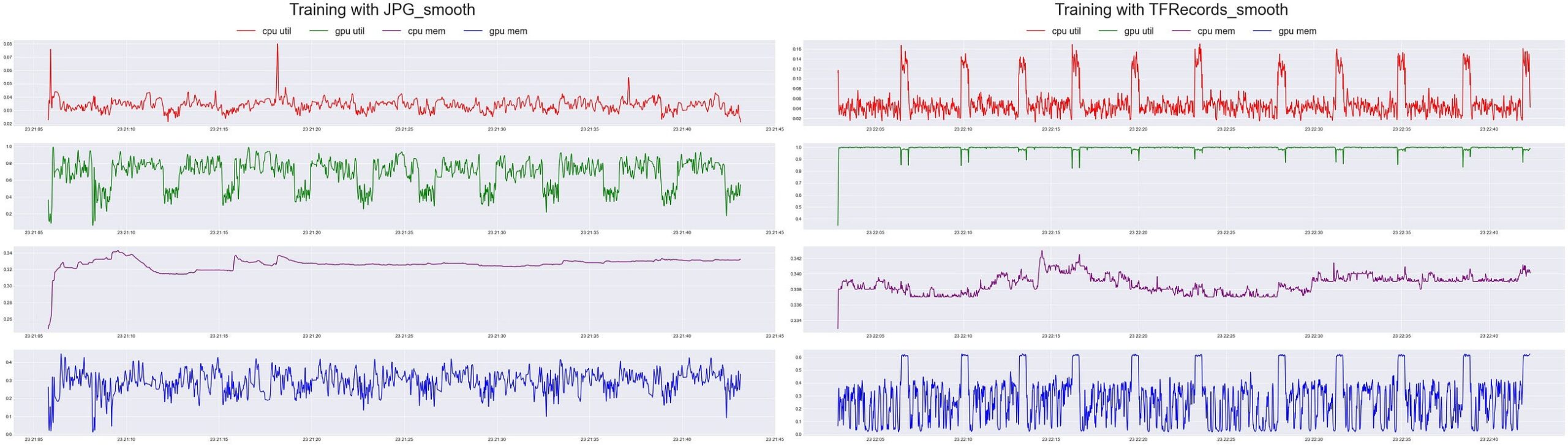
After smoothing, it’s very evident when a new epoch was starting while training with the TFRecords. There’s a 10 spaced out spikes in CPU Utilization that corresponds with 10 spikes in GPU memory utilization. This is clearly the CPU processing and loading the GPU with the next batches for the next epoch. This should be even more evident this is the case since we trained the model for 10 epochs, and there’s 10 spikes! Meanwhile, While training with the JPG images, there’s a lot of down time on the GPUs at each epoch. There’s 10 significant drops in GPU Utilization that appears to last for about a minute or so. Also it seems that the CPU is just taking its time processing the images.
Time distributions
Let’s now take a look at the distributions for the time it took to process each batch. One would assume that we shouldn’t see a significant difference in the time it takes to process a batch. This is because for both formats, they’re being converted to a (None, 299, 299, 3) tensor. Any differences between the two inputs would be purely due to stochasticity.
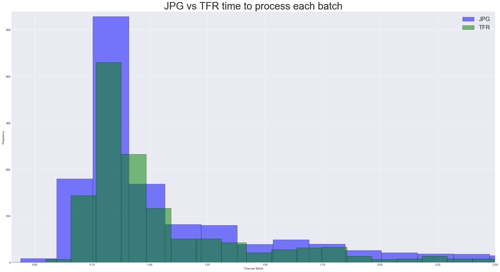
Sure enough this is what we see. The time to process each batch is more or less the same. The bit that would should be more interested in is the time for each epoch, since that involves the entire pipeline of the CPU and GPU processing. The distribution won’t be very interesting to look at since we only did 10 epochs. Hence setting the bins on the histogram to 3, this is what we have:
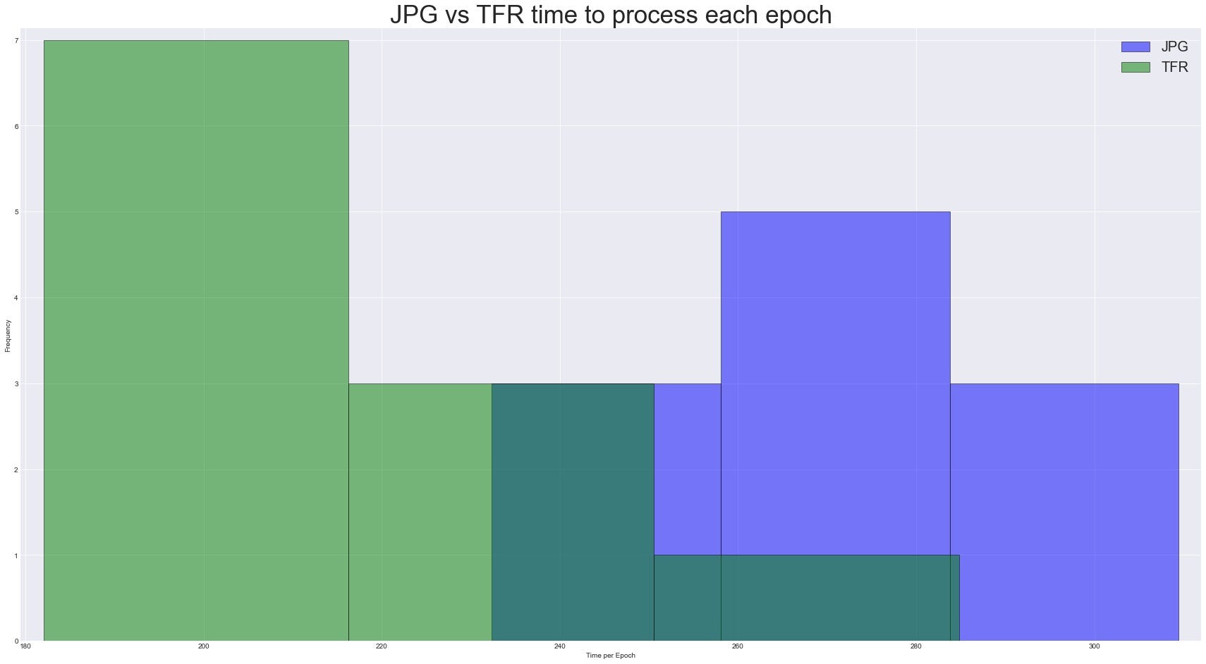
Although not a graph bountiful of data, it adds more context to what we already saw on Comet. The time spent per epoch is significantly less when training with TFRecords than with the raw data on disk. The data breaks down like:
Considering that it’s estimated to take 34 days to train ChatGPT with 1000 Nvidia A1000 GPUs, the nearly 80s difference between the two would add up very quickly to something significant.
