Image Inpainting for SDXL 1.0 Base Model + Refiner

Words By Abby Morgan

August 18, 2023

In this article, we’ll compare the results of SDXL 1.0 with its predecessor, Stable Diffusion 2.0. We’ll also take a look at the role of the refiner model in the new SDXL ensemble-of-experts pipeline and compare outputs using dilated and un-dilated segmentation masks. Finally, we’ll use Comet to organize all of our data and metrics. Feel free to follow along in the full-code tutorial here, or, if you can’t wait to see the final product, check out the public project here.

Realistic picture of an American astronaut in outerspace with planets and stars and meteorites and meteors in the background and a light halo around the astronaut. In the astronaut's helmet is the reflection of a fiery orange comet. "SDXL" is outlined in white in the background. — Image created by author with SDXL 1.0 base + refiner and edited in Canva; seed = -732, prompt = “astronaut in outerspace, photorealistic.”

Follow along with the Colab Create a free Comet account!

What is SDXL 1.0 and why should I care?

SDXL 1.0 is the new foundational model from Stability AI that’s making waves as a drastically-improved version of Stable Diffusion, a latent diffusion model (LDM) for text-to-image synthesis. As the newest evolution of Stable Diffusion, it’s blowing its predecessors out of the water and producing images that are competitive with black-box SOTA image generators like Midjourney.

A vertical bar chart showing the preference rates of users between SDXL 1.0 (base + refiner), SDXL 1.0 (base only) Stable Diffusion 1.5 and Stable Diffusion 2.0 — The results are in and practitioners prefer the SDXL 1.0 pipeline by a wide margin!

The improvements are the result of a series of intentional design choices, including a 3x larger UNet-backbone, more powerful pre-trained text encoders, and the introduction of a separate, diffusion-based refinement model. The refiner model improves the visual fidelity of samples using a post hoc image-to-image diffusion technique first proposed in SDEdit. In this tutorial, we’ll use SDXL with and without this refinement model to get a better understanding of its role in the pipeline. We’ll also compare these results with outputs from Stable Diffusion 2.0 to get a broader picture of the improvements introduced in SDXL.

Graphic of the SDXL 1.0 diffusion model architecture, including the base model and refiner model. — The SDXL 1.0 mixture-of-experts pipeline includes both a base model and a refinement model.

But these improvements do come at a cost; SDXL 1.0 involves an impressive 3.5B parameter base model and a 6.6B parameter refiner model, making it one of the largest open image generators today. This increase is mainly due to more attention blocks and a larger cross-attention context, since SDXL uses a second text encoder (OpenCLIP ViT-bigG with CLIP ViT-L).

SDXL 1.0 and the future

Still, the announcement is an exciting one! In the last year alone, Stable Diffusion has served as a foundational model in fields spanning 3D classification, controllable image editing, image personalization, synthetic data augmentation, graphical user interface prototyping, reconstructing images from fMRI brain scans, and music generation. SDXL 1.0 promises to continue Stable Diffusion’s tradition of widening the realm of generative AI possibilities.

In one incredible application of Stable Diffusion, researchers showed volunteers the top row of images above. They then fed fMRI scans of their brain activity to a Stable Diffusion model, which successfully created the bottom row of reconstruction images. — In one incredible application of a previous version of Stable Diffusion, researchers showed volunteers the top row of images above. They then fed fMRI scans of their brain activity to the model, which successfully created the bottom row of reconstruction images. What new advancements will SDXL bring?

SDXL 1.0 vs. the world

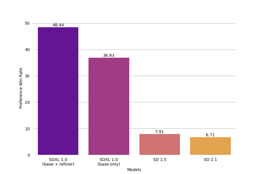
So, how does SDXL 1.0 fare in the wider world of text-to-image generative AI tools? According to SDXL, very well. In fact, it’s now considered the world’s best open image generation model. And while Midjourney still seems to have an edge as the crowd favorite, SDXL is certainly giving it a run for its money as a free open source alternative.

SDXL 1.0 is both open-source and open-access, meaning it’s free to use, as long as you have the computational resources to do so. But it doesn’t require much; all of the images in this article were generated using Google Colab’s A100 GPU. And according to Stability AI, SDXL 1.0 will even work effectively on consumer GPUs with just 8GB of VRAM, making generative text-to-image models more accessible than ever before.

But what makes SDXL image outputs better than ever? According to Stability AI, SDXL offers:

Better contrast, lighting and shadows
More vibrant and accurate colors
Native 1024 x 1024 resolution
Capacity to create legible text
Better human anatomy (hands, feet, limbs and faces)

We’ll explore some of these points in more detail below.

SDXL 1.0 for Model Explainability

Generative AI continues to find itself at the forefront of debates surrounding model explainability, transparency, and reproducibility. As AI becomes more advanced, model decisions can become nearly impossible to interpret, even by the engineers and researchers that create them. This is a particular concern with many state-of-the-art (SOTA) generative AI models, whose opacity limits our ability to wholly assess their performance, potential biases, and inherent limitations. So it comes as a commendable move towards model explainability and transparency that Stability AI has made SDXL an open model.

Image created using the SDXL 1.0 Stable Diffusion pipeline (base + refiner) of machine learning model explainability — Image created by author with SDXL base + refiner; seed = 277, prompt = “machine learning model explainability, in the style of a medical poster”

A lack of model explainability can lead to a whole host of unintended consequences, like perpetuation of bias and stereotypes, distrust in organizational decision-making, and even legal ramifications. What’s more, it hinders reproducibility, discourages collaboration, and restricts further progress. The decision to make Stable Diffusion models open source and open access follows a growing trend in the industry towards open artificial intelligence, which encourages practitioners to build upon existing work and contribute new insights.

Now, let’s try it for ourselves!

SDXL 1.0 in action

If you aren’t already, you can follow along with the full code in this Colab here. I should note that the code in this tutorial extends a pipeline I built in a previous article (which you can find here) but will also run as a standalone project if you’re eager to get started. To compare the performance of SDXL with Stable Diffusion 2.0, I’ll use the same images used in that tutorial. Because this article is not focused on image segmentation, I’ll also use the binary masks and image metadata generated in that project, which I uploaded to Comet as an Artifact for public use.

Although this tutorial functions as a standalone project, if you’re interested in how we created our initial segmentation masks and metadata, you can check out the first part of this project here:

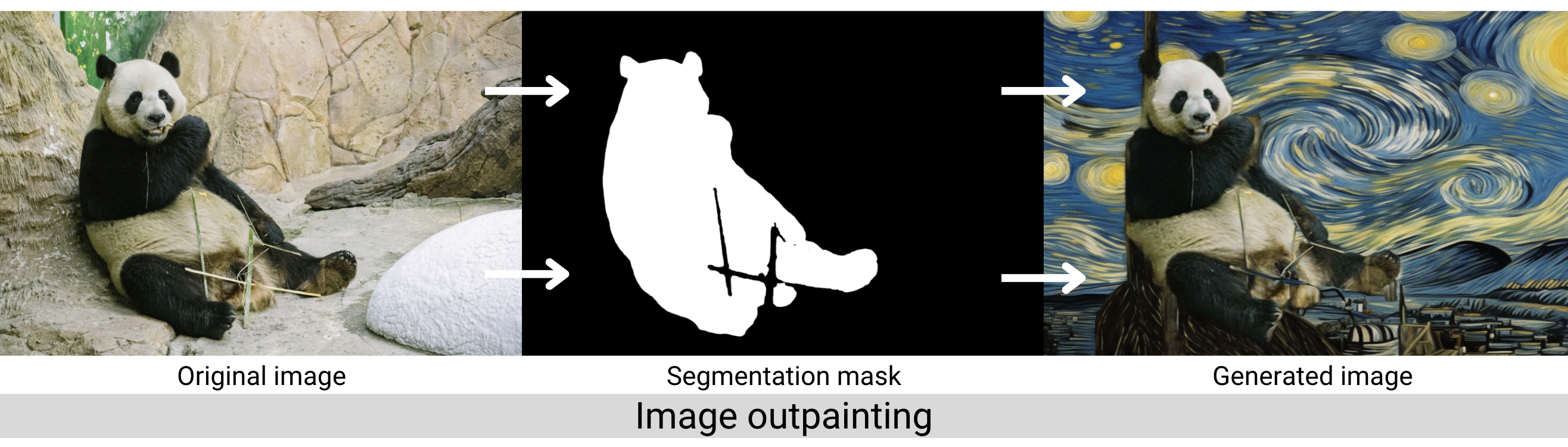
After we download the Artifact, we’ll perform image inpainting and outpainting using the SDXL Inpainting Pipeline from HuggingFace. We’ll use near-identical prompts to those used in the first part of this tutorial (with a few very minor exceptions).

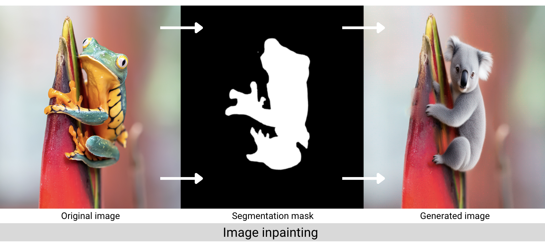
A graphic showing an original image, the segmentation mask of a frog, and the resulting inpatined image from the SDXL 1.0 diffusion pipeline. — Image inpainting refers to the process of filling-in missing data in a designated region of an image; graphic by author.

As a reminder, image inpainting is the process of filling in missing data in a designated region of an image. Outpainting is the process of extending an image beyond its original borders, which we’ll effectively do by inpainting the background masks of our images. The inpainting pipeline accepts both a positive and negative prompt, and we’ll set random seeds so you can produce the same results in your local environment.

Graphic of image outpainting showing an original input image of a panda, a segmentation mask, and the inpainted image resulting from the SDXL 1.0 diffusion model. — Image outpainting is the process of using generative AI to extend images beyond their original borders, thereby generating parts of the image that didn’t exist before; graphic by author.

Tracking our experiment

We’ll start off by instantiating a Comet Experiment so we can track our inputs, outputs, code, and other system metrics. You’ll need to grab your API key from your account settings. If you don’t already have an account, you can create one here for free.

Comet Artifacts

An Artifact is any versioned object arranged in a folder-like structure. In this way, Comet allows you to keep track of any data associated with the machine learning lifecycle. Our Artifact will be structured as follows:

The file folder structure of our image information (including segmentation masks) that we will download as a Comet Artifact. — By logging our Artifact to Comet and downloading to our local environment, we preserve its file structure; graphic by author.

Downloading an Artifact to your local environment is as simple as running the following code. If an Artifact isn’t in your personal workspace, make sure the owner of the Artifact has shared it with you or made it public (as in our example). Below we download the Artifact to our working directory, preserving its original file structure without any additional parsing.

Loading SDXL with Hugging Face

We’ll load the SDXL base model, refiner model, and inpainting pipelines from HuggingFace. We can do so with the following code:

Hyperparameters

Like any traditional machine learning model, SDXL has a variety of tunable hyperparameters that affect the quality of the output. We’ll cover some of the important ones here and keep track of which sets of values produced which outputs using Comet.

Unlike many traditional machine learning models, however, “quality” in this experiment is mostly subjective. And while there are some metrics to “objectively” assess the quality of images created by a generative model (see NRMSE, PSNR, SROCC and KROCC, ), there are issues with each of these metrics for inpainting, specifically. So, for this tutorial we’ll just be using ourselves as human assessors. And because of this, we’ll be relying heavily on our experiment tracking tool to trace which values led to which image outputs.

Let’s take a look at some of the important hyperparameters we’ll be setting.

Guidance scale

The guidance scale (also known as the classifier-free guidance scale or CFG scale) controls how similar the generated image will be to the original prompt. A lower guidance scale value allows the model more “creativity,” but images may become unrecognizable if it is set too low. A higher guidance scale value forces the generator to more closely match the prompt, but sometimes at the cost of image quality or diversity.

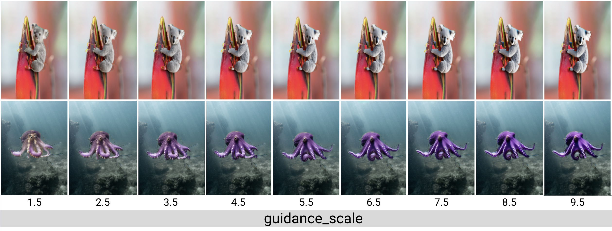
Guidance scale values typically fall in the range of 7-15, though Hugging Face suggests values between 7.5 and 8. For most images generated in this tutorial we will stick with the default value of 7.5.

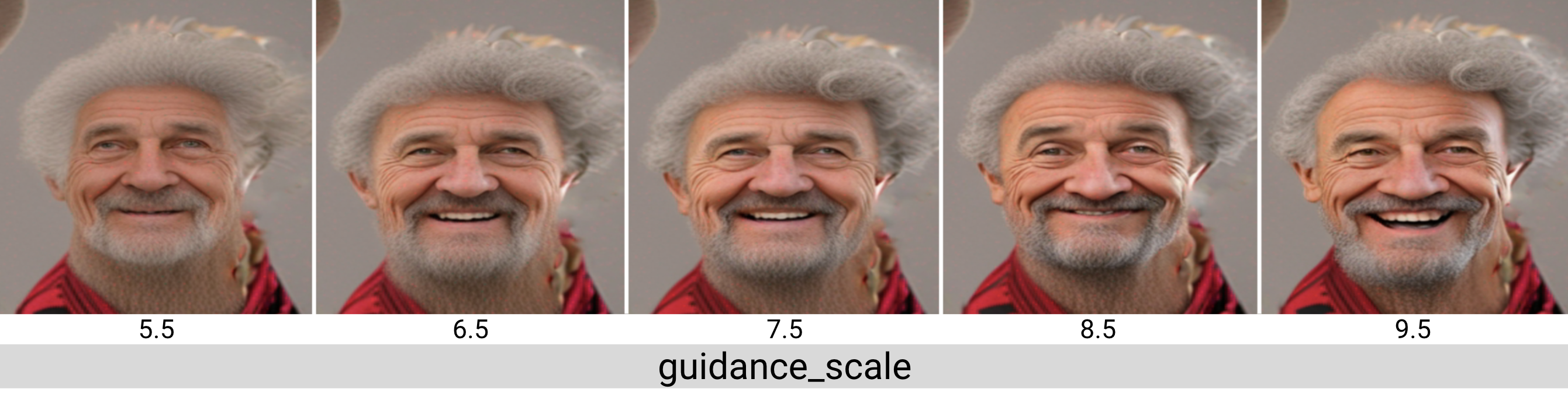
A picture of an old man with curly gray hair, on the left, slightly happy, becoming happier as you move right and the guidance scale increases. — The role of the guidance scale value becomes even clearer once we start to introduce subjective words, like feelings. How happy should the “happy man with curly hair” be? Graphic by author.

Most of our prompts are pretty objective (“a purple octopus”,”a red gummy bear”). But the role of the guidance scale value becomes even clearer once we start to introduce subjective words, like feelings. How happy should the “happy man with curly hair” be? We can see the model takes more liberty with this prompt as the guidance scale increases.

Number of inference steps

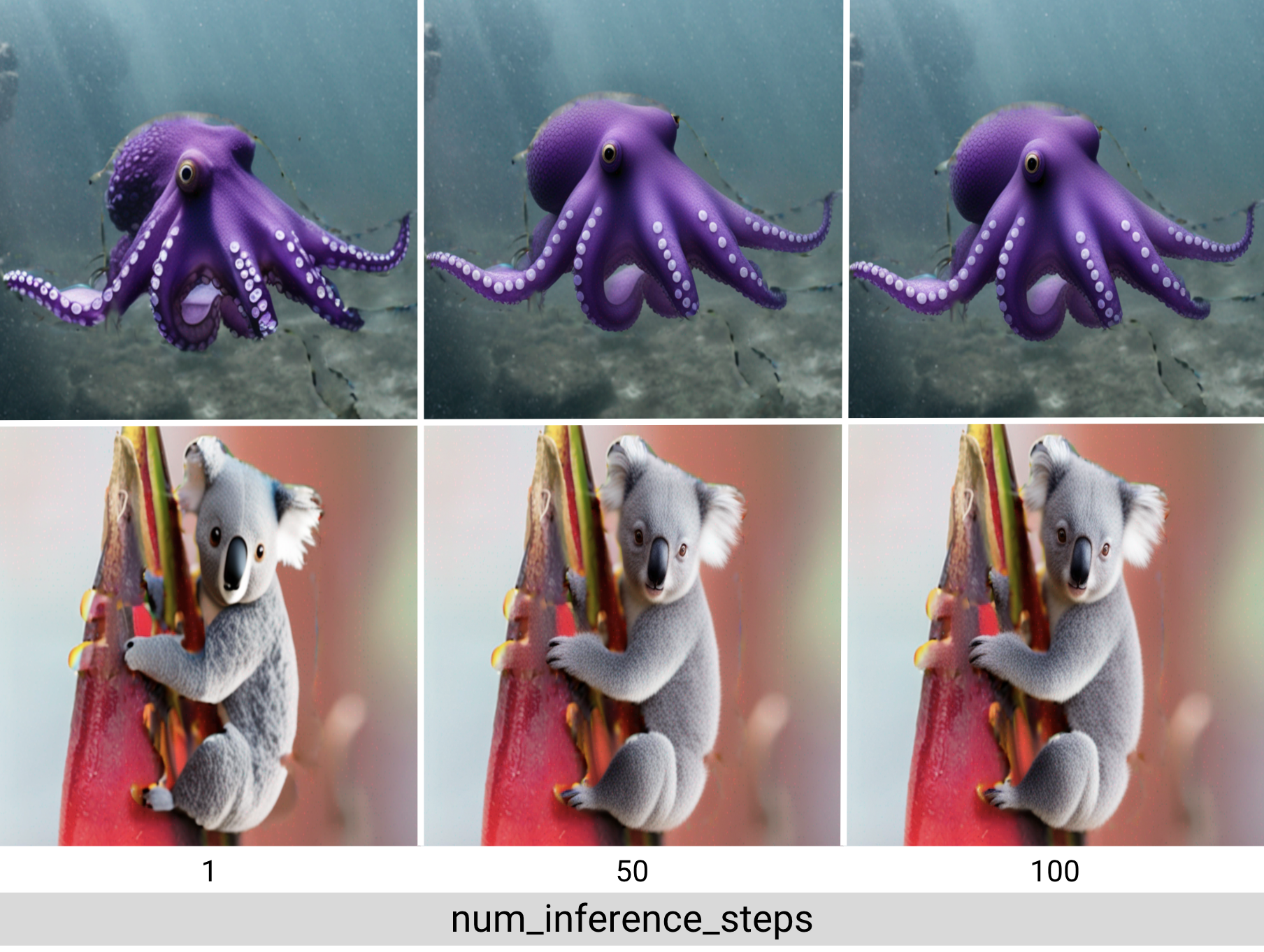
In general, the quality of the image increases with the number of inference steps, but as we can see in the image below, at a certain point the improvements become negligible. More inference steps also means the model takes longer to generate the image, which could become an issue for certain use cases. Stable Diffusion works very well with relatively few inference steps, so in this tutorial we’ll use around 70 inference steps per image.

Running SDXL 1.0 on different numbers of inference steps produces different results — The quality of the image generally increases with the number of inference steps, but more inference steps also means the model takes longer; graphic by author.

High noise fraction

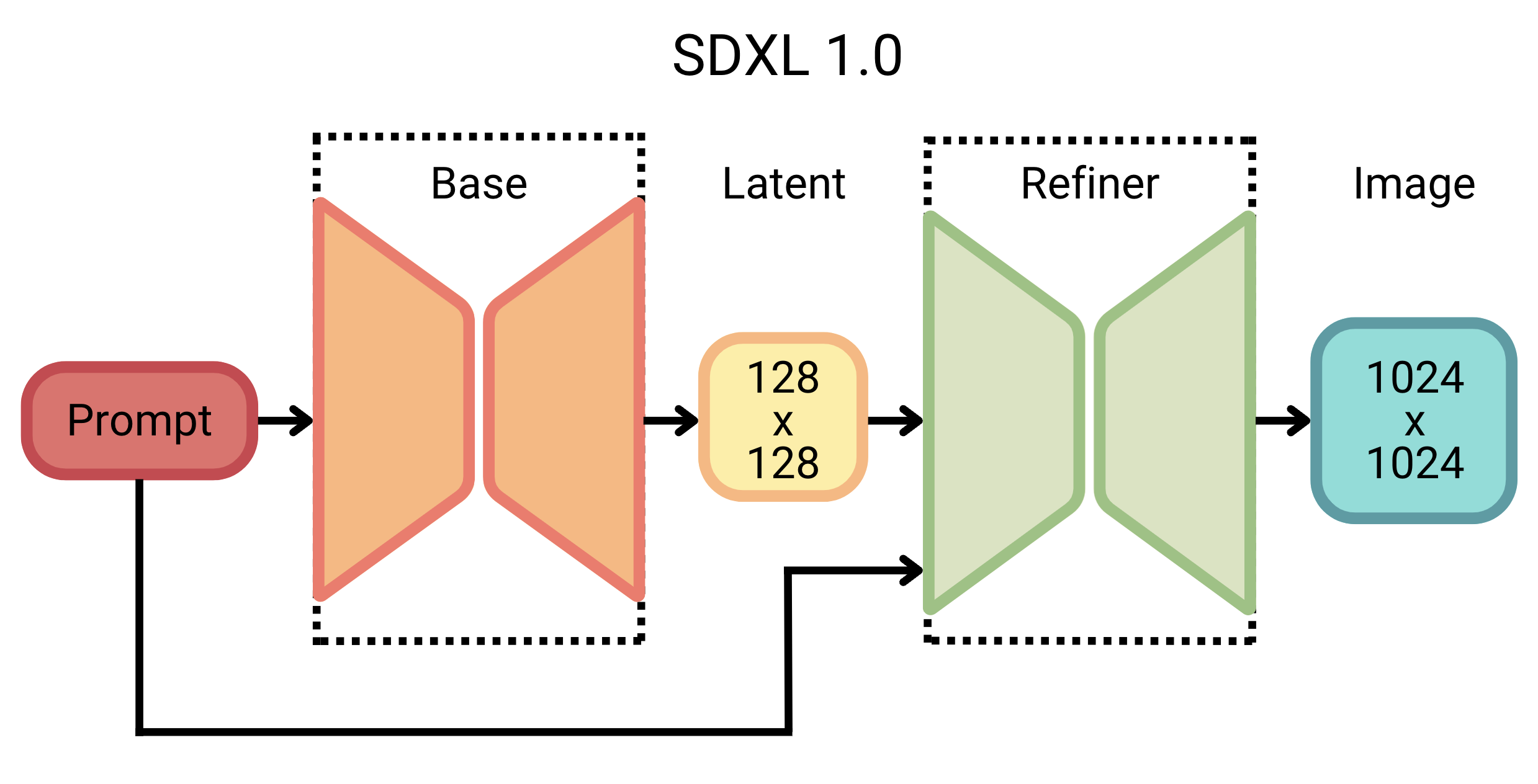
When using SDXL as a mixture-of-experts pipeline, as we are here, we’ll also need to specify the high noise fraction. The high noise fraction is the percentage of inference steps to run in each stage of the base model and refiner model. The base model will always serve as the expert for the high-noise diffusion stage and the refiner as the expert for the low-noise diffusion stage.

We set these inference intervals using the denoising_end parameter of the base model or the denoising_start parameter of the refiner model. Both are not needed, as they will always sum to 1. Each accepts a float between 0 and 1, representing the fraction of total inference steps for that model expert model.

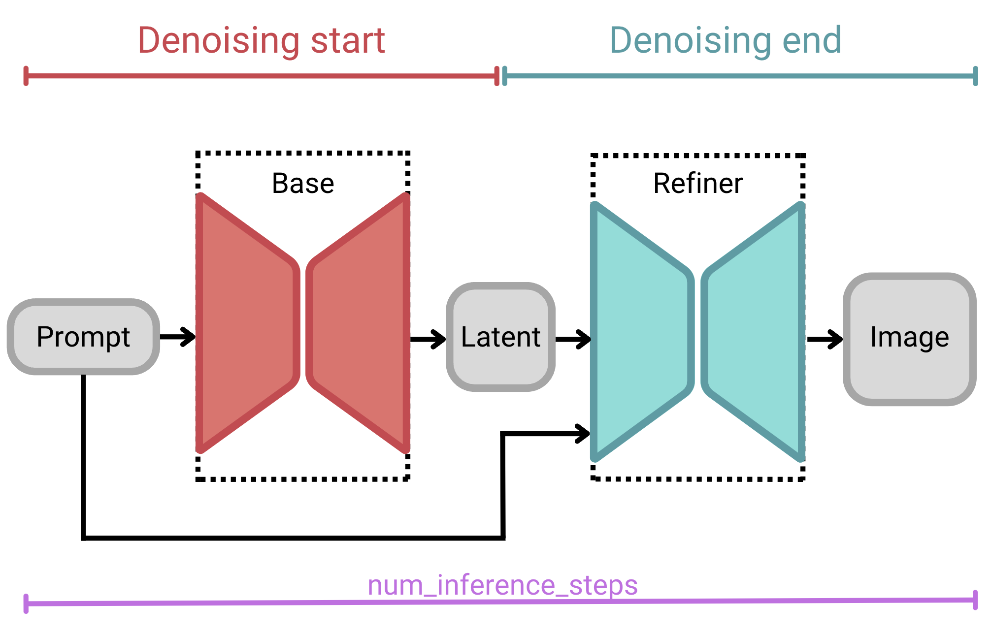
Graphic showing the SDXL 1.0 mixture-of-experts 2-stage architecture, demonstrating how the process is broken down into denoising start and denoising end. — The `high_noise_frac` or `denoising_start` is the percentage of inference steps that the model will run through the high-noise denoising stage (i.e., the base model); graphic by author.

For example, if we were to specify 100 total inference steps with a denoising_end of 0.7, then our input would iterate 70 steps in the base model and 30 steps in the refiner model. If we were to specify a denoising_end value of 0.9, on the other hand (with the same total inference steps), our input would iterate for 90 steps in the base model and 10 in the refiner model.

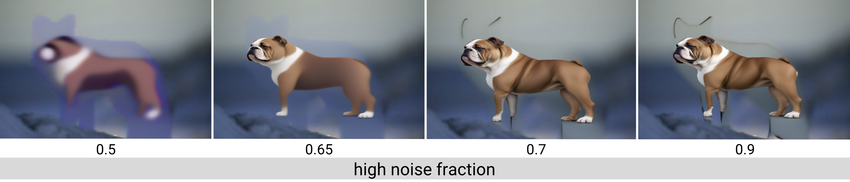
Image showing the effect of different high noise fraction or denoising values have on the output of the SDXL 1.0 pipeline — The high noise fraction, or `denoising_start`, values range from 0.0 to 1.0, but usually a value between 0.7 and 0.9 is appropriate; graphic by author.

This two-stage architecture makes SDXL especially robust, without sacrificing compute resources or inference time.

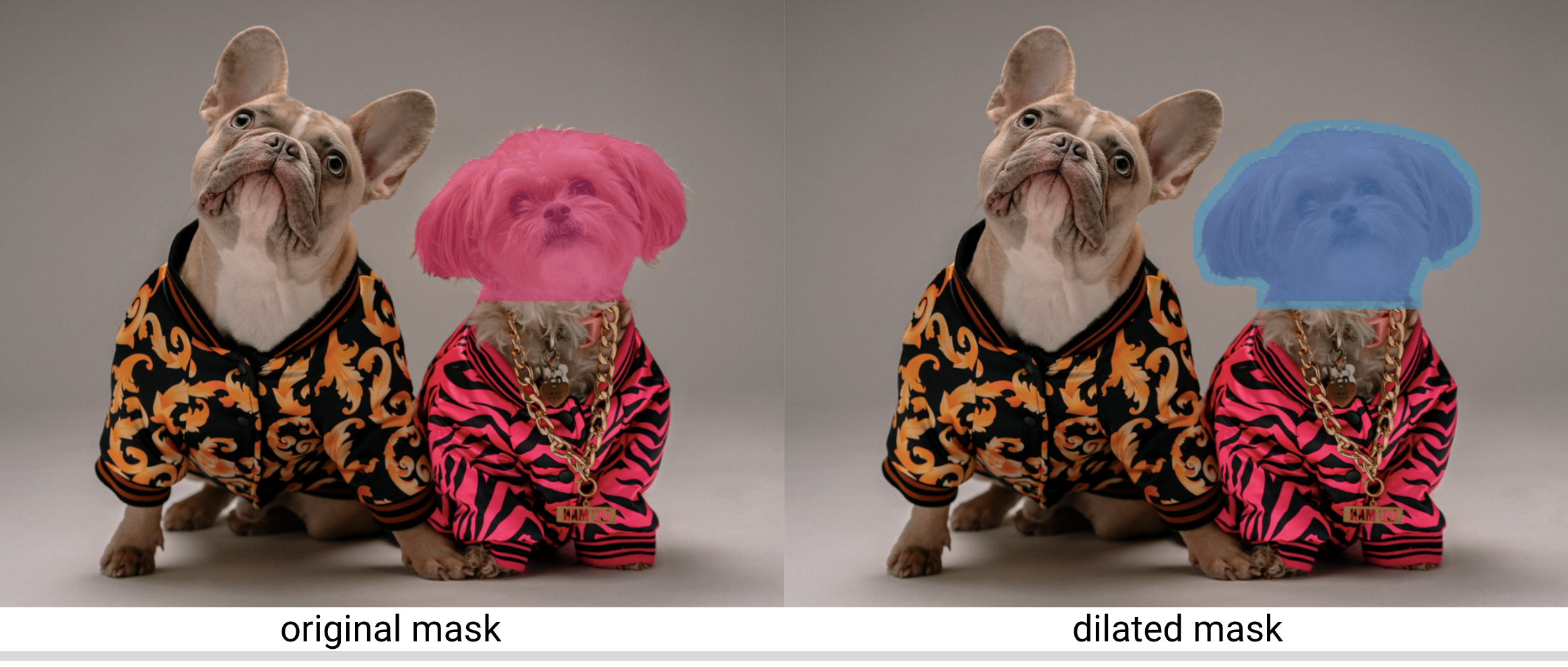
Kernel size and iterations

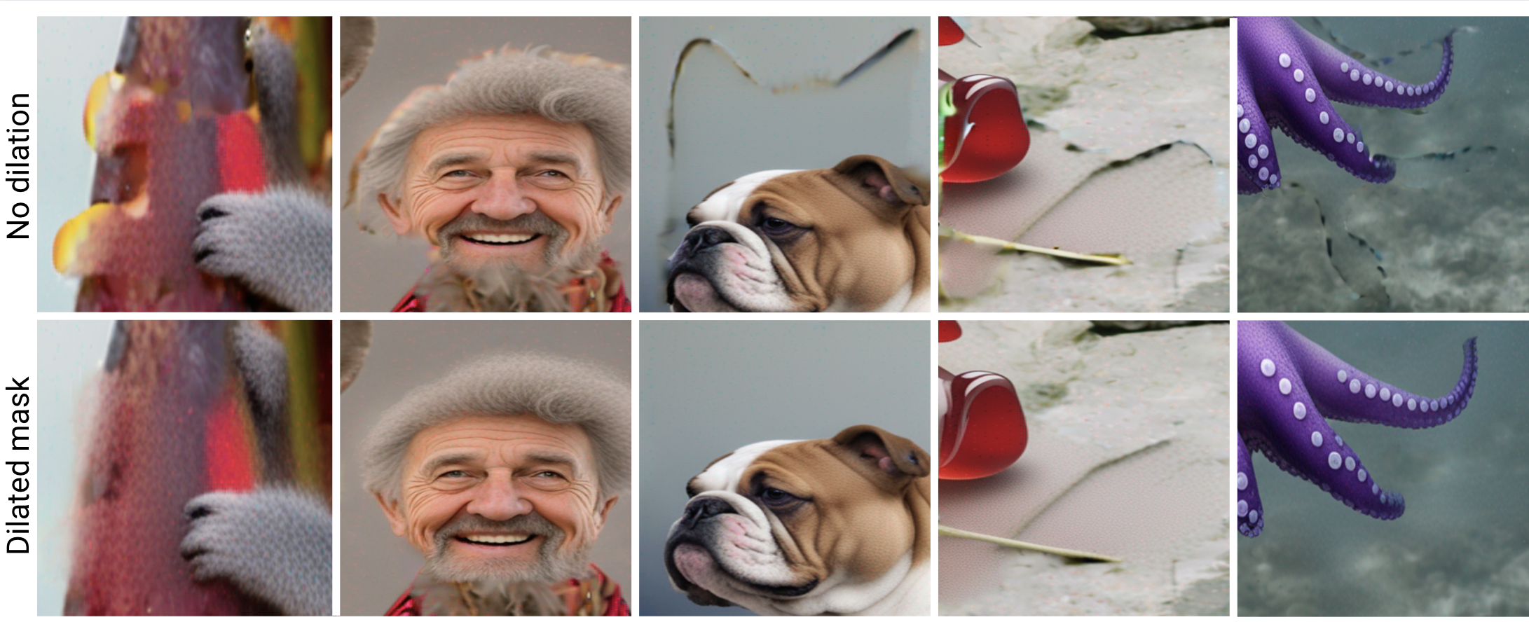
If we use masks that perfectly align with the object we are replacing, we might notice some awkward pixel transitions between the original image and where it was inpainted. By dilating the mask slightly and giving the inpainting pipeline access to background pixels near the inpainted object, the refiner can make a more seamless integration between the two.

Graphic showing the difference between a dilated segmentation mask and an un-dilated segmentation mask — Dilating the inpainting masks makes for a more seamless transition with the original background image; graphic by author.

In order to dilate the mask, we’ll need to set a kernel size and number of kernel iterations. These values may change depending on the image you are using. For more information on this process, see the docs from OpenCV. We’ll also define a function to simplify the dilation process:

Finally, how did I choose the random seeds? Well, randomly. I used random.randint(-1000,1000) and regenerated the images until I found an image I liked and wanted to work with. Then I kept tweaking hyperparameters using the same seed. That’s all!

Nested hyperparameters

In addition to the hyperparameters outlined above, we’ll also be logging a few others, including our prompts and negative prompts. Because we’ll be setting the same hyperparameters for our inpainting and outpainting pipelines, we’ll define our hyperparameters in nested dictionaries. For example:

These will be logged accordingly as nested hyperparameters in Comet, making them easier to access and organize, and helping to avoid duplication and confusion.

A GIF showing how nested hyperparameters are logged within the Comet ML UI — We use the same set of hyperparameters for our inpainting and outpainting pipelines, only with different values for each set. To avoid duplication or confusion, we log them as a nested dictionary and preserve this structure within the Comet UI.

Our SDXL 1.0 inpainting-outpainting pipeline

To stay consistent with the first part of this tutorial, for each of our five original input images, we generate both an inpainted, and an outpainted, image. For each of those examples, we’ll generate a sample using:

SDXL (base only)
SDXL (base + refiner)
SDXL (base + refiner + dilated masks)

We’ll then compare the results of these different methods to better understand the role of the refinement model and of dilating the segmentation masks. Once we’ve selected our best outputs, we’ll compare these with the best outputs from Stable Diffusion 2.0.

After writing a couple of functions to abstract away some of the noise, generating these samples (and logging them to Comet) will be as simple as the following lines of code.

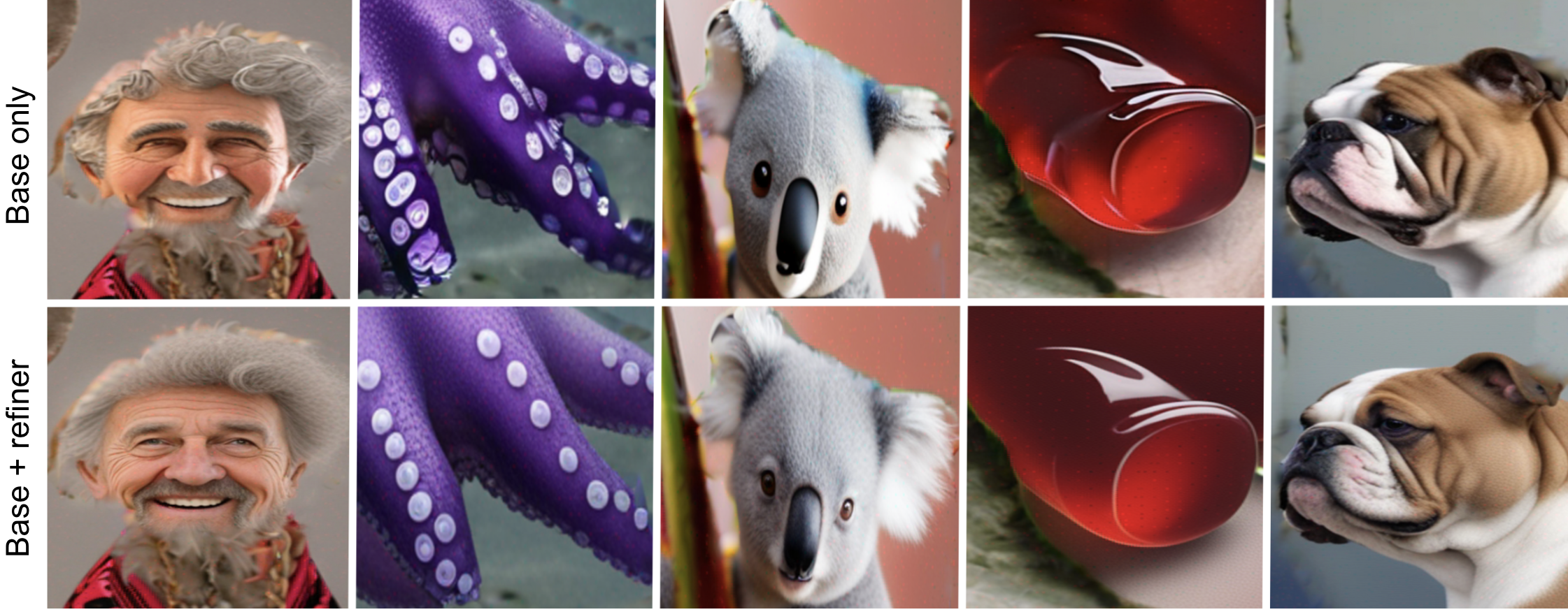
The refiner

Even at a quick glance, it’s pretty easy to see the role the refiner had in improving image quality. But the power of the SDXL refiner is most noticeable when you examine finer details like lines, textures, and faces. For this, it helps to take a closer look:

A graphic showing the same generated output images using only the SDXL 1.0 base model (top) and the SDXL 1.0 pipeline of base model + refiner — The power of the SDXL refiner is most noticeable when you examine finer details like lines, textures, and faces; graphic by author.

Dilated masks

Zooming in also helps us see the difference that dilating the masks made. The transitions between original background pixels and generated image are much smoother where masks have been dilated.

By zooming in, we can also see how dilating the segmentation masks helped smooth the transitions between original background pixels and generated image; graphic by author.

SDXL 1.0 results

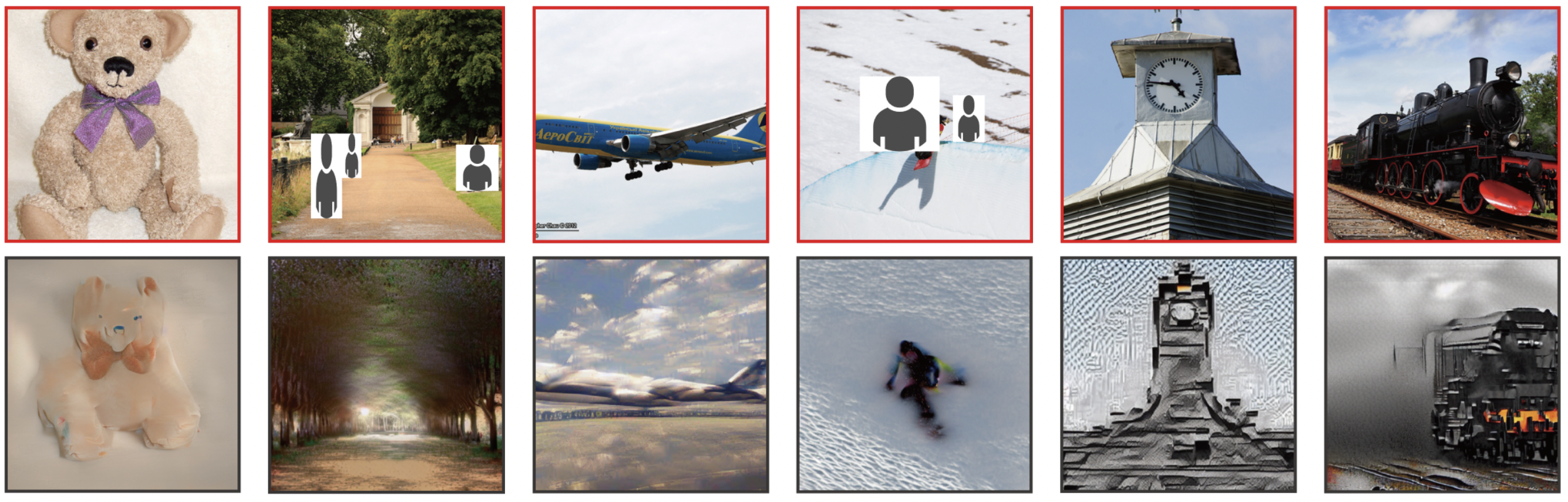
After all that hard work, how did SDXL 1.0 compare to Stable Diffusion 2.0? Let’s check out the results! First, our inpainted images:

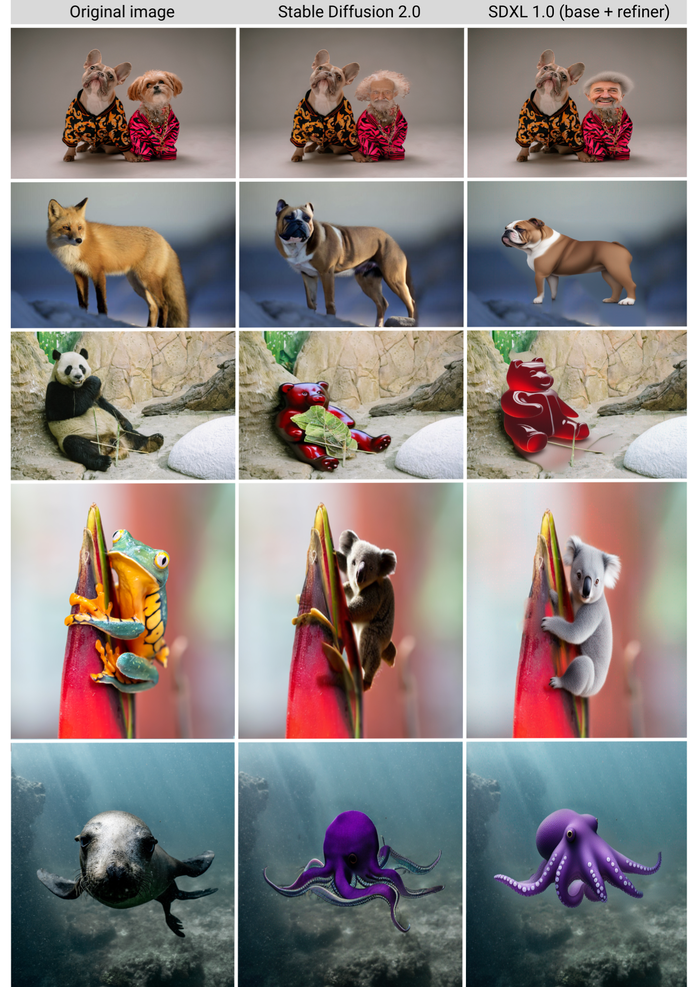
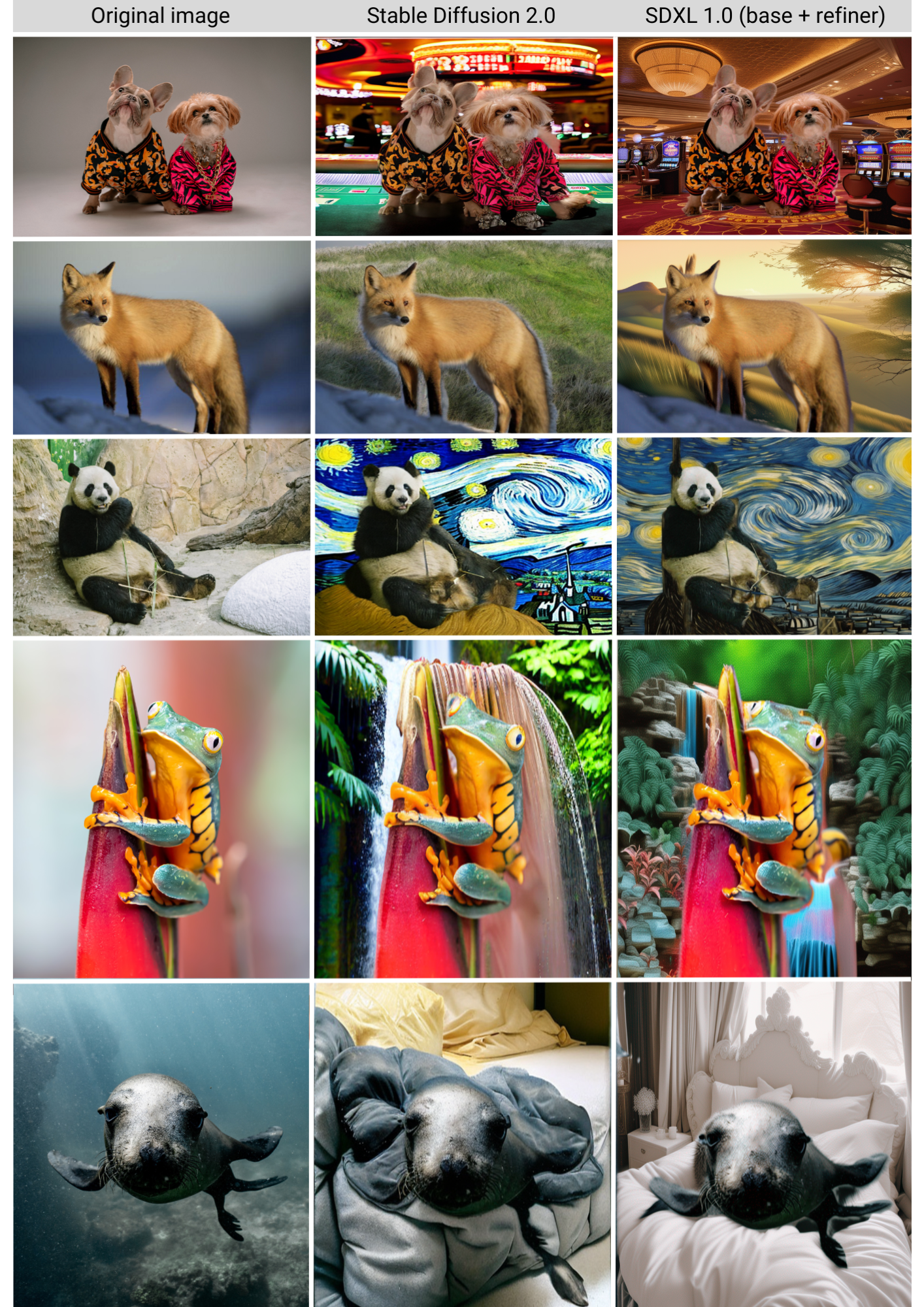
Comparing the results of Stable Diffusion 2.0 and SDXL 1.0 for image inpainting with the base + refiner models. — On the left, our original input images. In the center, the results of inpainting with Stable Diffusion 2.0. On the right, the results of inpainting with SDXL 1.0. I encourage you to check out the public project, where you can zoom in and appreciate the finer differences; graphic by author.

Clearly, SDXL 1.0 is a drastic improvement to Stable Diffusion 2.0! Now let’s check out our outpainting images (I encourage you to zoom in on the results to really see the finer differences too):

Comparing the results of inpainting with Stable Diffusion 2.0 with SDXL 1.0 base model + refiner. — On the left, our original input images. In the center, the results of outpainting with Stable Diffusion 2.0, and on the right the results of outpainting with SDXL 1.0. I encourage you to check out the public project, where you can zoom in and appreciate the finer differences; graphic by author.

Comparing our SDXL 1.0 results in Comet

As you can probably imagine, keeping track of which input images, prompts, masks, and random seeds were used to create which output images can get confusing, fast! That’s why we logged all of our images to Comet as we went.

Let’s head on over to the Comet UI now and take a look at each of our input images and the resulting output images after inpainting and outpainting:

Viewing our SDXL results in Comet with the Image Panel and Data Panel. — Viewing our results in Comet with the Image Panel and Data Panel.

We can also select individual experiments for comparison. This might be especially useful if we’re trying to reproduce an image that we experimented with multiple times, or if we’re trying to debug a particular experiment run.

Diffing our SDXL Stable Diffusion experiments in Comet — By diffing our experiments in Comet, we can visualize differences in code, hyperparameters, and other metrics. Also, we can view input and output data side-by-side.

Tracking our image prompts with Comet

We’ll also want to make sure to keep track of how we created each output so we can reproduce any of the results later on. Maybe we’ve run different versions of the same prompt multiple times. Or maybe we’ve tried different random seeds and want to pick our favorite result. By logging our prompts to Comet’s Data Panel, we can easily retrieve all the relevant information to recreate any of our image outputs.

A GIF showing how to log textual prompts for images in generative AI using Comet ML — With Comet’s Data Panels, we can filter and reorder columns, as well as sort rows by ascending or descending. Filtering can be especially helpful when looking for all prompts containing a particular keyword.

Conclusion

Thanks for making it all the way to the end, and I hope you found this SDXL tutorial useful! As a quick recap, in this article we:

Learned about the SDXL 1.0 base model and refiner model and compared outputs from each;
Explored the guidance_scale, num_inference_steps, and denoising_start hyperparameters;
Compared out image outputs across hyperparameter values, as well as;
Logged our nested hyperparameters to Comet;
Built an extensive dashboard in Comet to track, log, and organize our results.

For questions, comments, or feedback, feel free to connect with us on our Community Slack Channel. Happy coding!

Resources

FAQ

Where can I find the full code for this tutorial?

Find the full code in this Colab.

Where can I find the images used in this tutorial?

Download the dataset on Kaggle here. Download the segmentation masks and JSON metadata from Comet’s public example Artifacts here.

Can I use SDXL 1.0 with Clipdrop?

Yes, SDXL 1.0 is live on Clipdrop here.

Is SDXL 1.0 open-source and open-access?

Yes, SDXL 1.0 is open-source and open-access.

Where can I access the source code and model weights used in SDXL 1.0?

The SDXL 1.0 source code and model weights are available on Stability AI’s Github page here.

Can I access SDXL 1.0 via an API?

Yes, you can access SDXL 1.0 through the API here.

What image sizes should I use with SDXL 1.0?

According to Stable Diffusion Art, the recommended image sizes for the following aspect ratios are:

21:9 – 1536 x 640
16:9 – 1344 x 768
3:2 – 1216 x 832
5:4 – 1152 x 896
1:1 – 1024 x 1024

Can I use SDXL 1.0 on AWS SageMaker and AWS Bedrock?

Yes, you can use SDXL 1.0 on AWS SageMaker here and on AWS Bedrock here.

Is there an SDXL 1.0 Discord community?

Yes, the Stable Foundation Discord is open for live testing of SDXL models.

Is SDXL 1.0 available in Dreambooth?

Yes, Dreamstudio has SDXL 1.0 available for image generation.

Is SDXL 1.0 available with ControlNet?

Yes, try out the HuggingFace implementation here.

What license does SDXL 1.0 have?

SDXL 1.0 is released under the CreativeML OpenRAIL++-M License.

Where can I find the complete Comet project?

Explore the public Comet project here.

Where can I create a Comet account?

Where can I ask for help with Comet?

For questions, comments, or feedback, please join our Community Slack to chat with fellow practitioners and Comet employees!

Abby Morgan

AI/ML Growth Engineer @ Comet