Sentiment analysis, commonly referred to as “opinion mining,” is the method of drawing out irrational information from written or spoken words. The study of how people communicate their thoughts, beliefs, and feelings through language is a fast-expanding area of natural language processing (NLP).

Customer service, marketing, and political analysis are just a few of the many uses for sentiment analysis. Companies can use sentiment analysis in customer service, for instance, to monitor and address client feedback and grievances posted on websites, social media platforms, and other channels. They can use this to enhance the consumer experience and pinpoint areas where their goods or services need to be improved.

In marketing, businesses can utilize sentiment analysis to comprehend consumer perceptions of their brand, those of their rivals, and market trends. They can use this information to adapt their marketing plans so that they more closely match the interests and demands of their target market.

Sentiment analysis is often applied to political analysis. Sentiment analysis is a tool that political scientists and analysts can use to monitor and examine public opinion on political issues, politicians, and parties. This can offer insightful information on the attitudes and beliefs of voters and aid in the prediction of election results.

There are several methods for performing sentiment analysis, including rule-based approaches, lexicon-based approaches, and machine-learning approaches.

In rule-based techniques, the text is classified as positive, negative, or neutral by creating a set of rules or heuristics. These criteria may be based on language elements such as keywords, grammar, or other aspects. Although this technology is quick and easy to use, it is error-prone and might not be able to fully capture the subtleties of human language.

Lexicon-based strategies make use of a pre-established collection of words that are connected to either positive or negative emotion. The quantity of positive and negative words in a passage of text can be used to gauge its mood. Although this strategy is more precise than rule-based ones, it is constrained by the scope and standard of the vocabulary that is being utilized.

A machine learning model is trained using a sizable dataset of text that has been labeled in order to classify language as positive, negative, or neutral. These models are more accurate than rule-based or lexicon-based methods because they can learn to recognize patterns and features that are indicative of sentiment. But they need a lot of labeled training data, and the dataset could be biased.

In this article, we’ll learn how to link Comet with Disneyland Sentiment Analysis. In order to accomplish this, we will perform some EDA on the Disneyland dataset, and then we will view the visualization on the Comet experimentation website or platform. Let’s get started!

About Comet

Comet is an experimentation tool that helps you keep track of your machine-learning studies. Another significant aspect of Comet is that it enables us to carry out exploratory data analysis. Comet’s interoperability with well-known Python visualization frameworks enables us to achieve our EDA goals. You can learn more about Comet here.

Prerequisites

If the Comet library isn’t currently installed on your machine, you can add it by entering one of the following commands at the command prompt. Be aware that pip is probably what you should use if you’re installing packages directly into a Colab notebook or another environment that makes use of virtual machines.

pip install comet_ml

— or —

conda install -c comet_ml

We then create our .comet.config file and add in our API key, workspace, and name of our project so all the readings on our models can be automatically tracked and logged. If you don’t already have a Comet account, you can sign up for free here, and then just grab your API key from Account settings / API Keys.

The Analysis

In this lesson, we’ll walk you through the process of running sentiment analysis on reviews of Disneyland and then explore the results with Comet. Specifically, we’ll be using the Disneyland dataset from Kaggle, which is a sizable dataset. Simply determining whether or not people are truly happy at Disneyland is the sole purpose of this analysis.

The first step involves loading your Comet libraries and other Comet-related dependencies, and the importance of this is that it captures all your readings automatically from start to finish.

from comet_ml import Experiment
comet_string = """[comet] 
api_key=K1fGCe5YL4XrwI01qoCSNvY3R
project_name=Sentiment Analyis 
workspace=olujerry
"""
with open('.comet.config', 'w') as f:
    f.write(comet_string)

Step 2: Import and install all libraries and dependencies.

import numpy as np
import pandas as pd
import matplotlib.pyplot as plt
import seaborn as sns
color = sns.color_palette()
%matplotlib inline
import plotly.offline as py
py.init_notebook_mode(connected=True)
import plotly.graph_objs as go
import plotly.tools as tls
import plotly.express as px

Step 3: Load the dataset.

Disney_reviews = pd.read_csv('/content/DisneylandReviews.csv',encoding='latin-1')

Step 4: Perform some EDA on the dataset.

Disney_reviews.head()

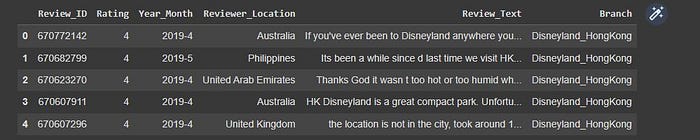
We can see that the dataframe contains some ratings, year, month, reviewer’s location, and then the reviews.

The data that we will be using most for this analysis is “rating,” “Review_Text,”and “Branch.”

1. Review_ID: unique id is given to each review
2. Rating: ranging from 1 (unsatisfied) to 5 (satisfied)
3. Year_Month: when the reviewer visited the theme park
4. Reviewer_Location: country of origin of the visitor
5. Review_Text: comments made by the visitor
6. Disneyland_Branch: location of Disneyland Park

Step 5: Deeper EDA

Now, we will take a look at the variable “Rating” to see if the majority of the customer ratings are positive or negative.

fig = px.histogram(Disney_reviews, x="Rating")
fig.update_traces(marker_color="turquoise",marker_line_color='rgb(8,48,107)',
                  marker_line_width=1.5)
fig.update_layout(title_text='Disneyland Ratings')

From here, we can tell that the majority of client reviews are favorable. This makes me think that most reviews will be largely favorable as well, which will be examined after some time.

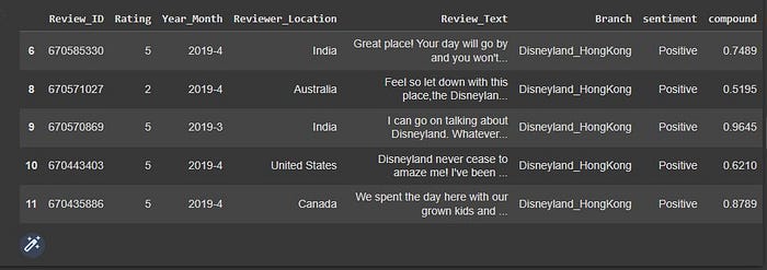
Using a module called VADER (Valence Aware Dictionary for Sentiment Reasoning), text sentiment analysis can be sensitive to both the polarity (positive/negative) and intensity (strong) of emotion. It is specifically created for attitudes expressed through social media and applied directly to unlabeled text data. The sentiment intensity analyzer function of VADER accepts a string and produces a dictionary of scores for each of the following categories: negative neutral positive compound (the total of the negative, neutral, and positive scores, adjusted between -1 and +1) (strongly positive).

Have you tried Comet? Sign up for free and easily track experiments, manage models in production, and visualize your model performance.

Scores can vary between -1 and 1, with -1 being very negatively skewed and +1 being very positively skewed. The compound score will be used to determine whether or not Disneyland-related reviews are favorable or unfavorable.

The sentiment intensity analyzer will now be initialized, and a lambda function will be created that accepts a text string, and runs the Vader. polarity scores() method on it to obtain the results, and then returns the compound scores. We may add a new compound column to the data frame containing all the compound scores for each review by using Pandas’ apply function.

from nltk.sentiment.vader import SentimentIntensityAnalyzer
import nltk
nltk.download('vader_lexicon')
vader = SentimentIntensityAnalyzer()

# Apply lambda function to get compound scores.
function = lambda title: vader.polarity_scores(title)['compound']
Disney_reviews['compound'] = Disney_reviews['Review_Text'].apply(function)
Disney_reviews.head(5)

Step 5: Visualizing Sentiments

Let’s examine the distribution of feelings. By generating word clouds, we may better comprehend the frequently used terms. A word cloud often referred to as a text cloud, is a visual representation in which a word gets bigger and bolder the more frequently it appears in the text.

Let’s use the word cloud plot to visualize every word in the data.

from wordcloud import WordCloud
import seaborn as sns
import matplotlib.pyplot as plt

allWords = ' '.join([twts for twts in Disney_reviews['Review_Text']])
wordCloud = WordCloud(width=500, height=300, random_state=21, max_font_size=110).generate(allWords)

plt.imshow(wordCloud, interpolation="bilinear")
plt.axis('off')
plt.show()

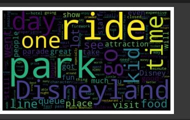
We can see that “ride,” “park,” “Disneyland,” “time,” and “day” are the common words that stand out.

The next step is to add a new column to our data frame called sentiment and to construct a function to calculate the negative (-1), neutral ((0), and positive (+1) feelings.

def getAnalysis(Rating):
 if Rating < 0:
    return 'Negative'
 elif Rating == 0:
    return 'Neutral'
 else:
    return 'Positive'

Disney_reviews['sentiment'] = Disney_reviews['compound'].apply(getAnalysis)

Disney_reviews.head(5)

Let’s look at the counts for each sentiment type.

Disney_reviews['sentiment'].value_counts()

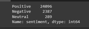
From the info, we can see that the positive numbers are higher than the negatives, which shows that people are really happy about their experience at Disneyland.

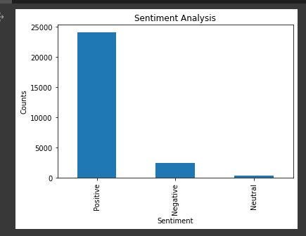
plt.title('Sentiment Analysis')
plt.xlabel('Sentiment')
plt.ylabel('Counts')
Disney_reviews['sentiment'].value_counts().plot(kind = 'bar')
plt.show()

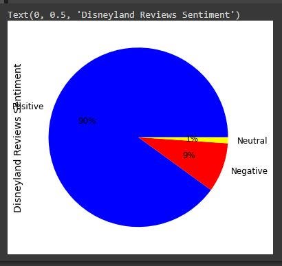
Visualize the distribution of sentiments across all reviews.

Disney_reviews.sentiment.value_counts().plot(kind='pie', autopct='%1.0f%%',  fontsize=12, figsize=(9,6), colors=["blue", "red", "yellow"])
plt.ylabel("Disneyland Reviews Sentiment", size=14)

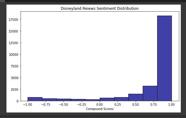
Visualize sentiment distribution based on compound scores.

plt.figure(figsize=(8, 5))
sns.histplot(Disney_reviews, x='compound', color="darkblue", bins=10, binrange=(-1, 1))
plt.title("Disneyland Reiews Sentiment Distribution")
plt.xlabel("Compound Scores")
plt.ylabel("")
plt.tight_layout()

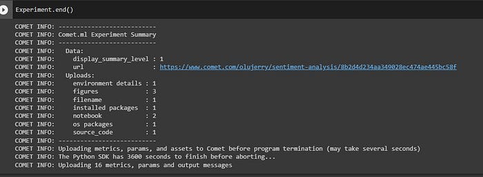
Step 6: Visualizing Results in Comet

After running the sentiments, it’s time to view our logged visualization in Comet, and from there we can perform further experiments and also get further insights. So to view the logged visuals, we have to end the experiment.

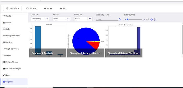
We then go further and perform more experiments on our sentiment analysis.

There were 100 reviews in all. The overwhelming majority of evaluations are favorable about Disneyland. 90% of the opinions are positive, 9% are negative, and 1% are neutral. These findings lead me to believe that Disneyland will undoubtedly be a wonderful destination to come and unwind.

Thank you for reading; you can find the complete tutorial code here.