At its core, the discipline of Natural Language Processing (NLP) tries to make the human language “palatable” to computers. Many data we analyze as data scientists consist of a corpus of human-readable text. Before we can feed this data into a computer for analysis, we must preprocess it.

In this article, let’s dive deep into the Natural Language Toolkit (NLTK) data processing concepts for NLP data. Before building our model, we will also see how we can visualize this data with Kangas as part of exploratory data analysis (EDA).

Ultimately, we will create an Email Spam Classifier with TensorFlow and the Keras API and track it with Comet. In the meantime, if you need to become more familiar with Comet, check out their incredible platform here.

Getting started with the NLTK library

NLTK offers excellent tools for developing Python programs that leverage natural language data. It has several text-processing libraries for tokenization, stemming, part-of-speech tagging, semantic reasoning, and many more tasks.

To start using NLTK, you need to install it. To do this, just run pip install nltkin your command line or !pip install nltk if using an interactive notebook.

Tokenization

Tokenization, also referred to as lexical analysis, is common practice in NLP. It involves splitting text data into lexical tokens, which allow us to work with smaller pieces of text (phrases, sentences, words, or paragraphs) that are still relevant, even once separated from the rest of the text. A tokenizer is responsible for this process.

There are two ways we can tokenize our text data with NLTK. We can either:

• Tokenize by word.
• Tokenize by sentence.

Tokenize by word

Here, we break down the text into individual words. Among other things, this can help identify frequently occurring words for a given analysis.

NLTK provides word_tokenizer that allows us to split text into words. Let’s see how:

import nltk
from nltk.tokenize import word_tokenize

# Text to tokenize
text_example = """We can do so much with Natural Language Processing ranging 
from speech recognition, recommendation systems, spam classifiers, and so 
many more applications."""

# Tokenizing
word_tokenized_sent = word_tokenize(text_example.casefold())
print(word_tokenized_sent)

# RESULTS
'''

['we', 'can', 'do', 'so', 'much', 'with', 'natural', 'language', 
'processing', 'ranging', 'from', 'speech', 'recognition', ',', 
'recommendation', 'systems', ',', 'spam', 'classifiers', ',', 
'and', 'so', 'many', 'more', 'applications', '.']

'''

Notice that we used casefold() on the text_example. The method ignores whether the letters in the text are uppercase or lowercase and treats all as lowercase. Alternatively, we could use text_example.lower() to convert the text into lowercase.

We must convert the text data into lowercase so all words are in the same case. If this is avoided, the model could interpret words like stock, Stock, and STOCK as unique tokens.

Tokenize by sentence

When we have text with multiple sentences, we can break them into a list of individual sentences.

from nltk.tokenize import sent_tokenize

text_example2 = """We can do so much with Natural Language Processing ranging from
speech recognition, recommendation systems, spam classifiers, and so many more applications.
These applications also leverage the power of Machine Learning and Deep Learning.
"""

sentence_tokenized= sent_tokenize(sentences_example.casefold())
print(sentence_tokenized)

# RESULTS 
'''

['we can do so much with natural language processing ranging from speech recognition, recommendation systems, spam classifiers, and so many more applications.',
 'these applications also leverage the power of machine learning and deep learning.'

'''

With sentence tokenizing, we get a list of two sentences from the text.

Removing stop words

In most cases, this operation occurs after we tokenize the data. Stop words are words that only add to the fluidity of text or speech but contain no meaningful information relevant to our task or the text itself.

First, we need to download and import the stop words that are provided by NLTK. Alternatively, we can also define our own stop words, but for this example the default list is more than sufficient.

Let’s use our word tokenized sentence above:

nltk.download('stopwords') # download the stopwords from nltk
from nltk.corpus import stopwords

# get stopwords in english
eng_stopwords= stopwords.words('english')

# filter stopwords with list comprehension
tokens_no_stopwords = [word for word in word_tokenized_sent if word not in stopwords_eng]
print(tokens_no_stopwords)

# RESULTS
'''

['much', 'natural', 'language', 'processing', 'ranging', 'speech', 'recognition', 
',', 'recommendation', 'systems', ',', 'spam', 'classifiers', ',', 'many', 
'applications', '.']

'''

Notice the disappearance of stop words like ‘do’, ‘so’, ‘from’ etc.

Stemming

Stemming is where we reduce words to their base form or root form, like cutting down tree branches to their stem. Stemming normalizes text and makes processing easier for Information Retrieval (IR) or text mining tasks.

A stemmer will apply rules that remove suffixes and prefixes from a word and reduce it to its root. This, in turn, reduces the time complexity and space. There are various types of stemming algorithms:

• Porter Stemmer: We mostly use this algorithm for its speed, minimal error rate, and simplicity. It is based on the fact that suffixes in the English language are composed of smaller and simpler suffixes. It is only limited to English words. Import as: from nltk.stem.porter import PorterStemmer.
• Snowball stemmer: This is a multilingual stemmer. Thus, it supports other languages. It is more aggressive than the Porter stemmer. Import as: from nltk.stem import SnowballStemmer.
• Lancaster stemmer: Despite being more aggressive and dynamic than the other stemmers, it is confusing when small words are involved. This stemmer is also less efficient. Import as: from nltk.stem.lancaster import LancasterStemmer.

We will use the Porter stemmer as the commonly preferred choice. The approach is similar if you choose to use the other stemmers, that is, based on what model you are building.

We will feed the stemmer the tokens_no_stopwords list derived from removing the stop words section.

from nltk.stem.porter import PorterStemmer

# Create a stemmer object
stemmer = PorterStemmer()

# Stemming
stemmed_tokens = [stemmer.stem(token) for token in tokens_no_stopwords]

print(f"===Unstemmed tokens==== {tokens_no_stopwords}")
print(f"===Stemmed tokens==== {stemmed_tokens}")

# RESULTS
'''

===Unstemmed tokens====
 ['much', 'natural', 'language', 'processing', 'ranging', 'speech', 'recognition', 
  ',', 'recommendation', 'systems', ',', 'spam', 'classifiers', ',', 'many', 'applications', '.']

===Stemmed tokens====
 ['much', 'natur', 'languag', 'process', 'rang', 'speech', 'recognit', ',', 'recommend', 
  'system', ',', 'spam', 'classifi', ',', 'mani', 'applic', '.']

'''

Notice how the words were cut. It is easy to notice that the resultant words are a bit confusing and appear meaningless. This poses one of the negative effects of stemming. The readability of the text is compromised, and in some cases, it may not even produce the correct root form of the word.

A stemmer can also produce inconsistent results. Let’s look at an example:

some_txt = "Discovering the wheel is among the best scientific discoveries ever made."

def stem_text(text):
    token_lst = word_tokenize(some_txt.casefold())
    token_no_stpw = [word for word in token_lst if word not in eng_stopwords]
    inco_stemmed_tokens = [stemmer.stem(token) for token in token_no_stpw]
    
    return inco_stemmed_tokens

# RESULT
'''

['discov', 'wheel', 'among', 'best', 'scientif', 'discoveri', 'ever', 'made', '.']

'''

We notice that the words ‘Discovering’ and ‘discoveries’ do not end up in the same base form (discover). There are two main errors we could encounter while stemming:

• Over-stemming (False positives): Occurs when the stemmer produces different base forms of two related words that should share a base form.
• Under-stemming (False negatives): When two unrelated words stem to the same base form while they should not.

In most cases, the above errors can be caused by the following:

• When the stemmer is too aggressive.
• When the stemmer does not consider the context of the text.
• When the stemmer in use is not designed for the particular language.

To get around these errors, we could use Lemmatizers instead of stemmers.

Hang on for lemmatization!

Part of speech (PoS) Tagging

Part of speech tagging involves labeling the words in the text data according to their part of speech. These parts of speech include:

• Noun (labeled with NN tag)
• Pronoun (labeled with PRP tag)
• Adjective (labeled with JJ tag)
• Verb (labeled with VB tag)
• Adverb (labeled with RB tag)
• Preposition
• Conjunction
• Interjection

To see all available tags and their meanings run:

nltk.download('averaged_perceptron_tagger')
nltk.download('tagsets')
nltk.help.upenn_tagset()

Let’s use the tokens_no_stopwords list derived from removing the stop words section and tag parts of speech.

pos_tagged_tokens = nltk.pos_tag(tokens_no_stopwords)
print(pos_tagged_tokens)

# RESULTS
'''

[('much', 'JJ'), ('natural', 'JJ'), ('language', 'NN'), ('processing', 'NN'), 
 ('ranging', 'VBG'), ('speech', 'NN'), ('recognition', 'NN'), (',', ','), 
 ('recommendation', 'NN'), ('systems', 'NNS'), (',', ','), ('spam', 'JJ'), 
 ('classifiers', 'NNS'), (',', ','), ('many', 'JJ'), ('applications', 'NNS'), 
 ('.', '.')]

''' 

An example of where PoS tagging would be applicable is when there is a need to know a product’s qualities in a review. In this case, we could tag the tokenized data, extract all the adjectives, and evaluate the review’s sentiment.

Standardizing model management can be tricky but there is a solution. Learn more about experiment management from Comet’s own Nikolas Laskaris.

Lemmatizing

This is similar to stemming, but with a significant difference. Unlike stemming, lemmatizing produces words to their root form but returns a complete English word (as would appear in a dictionary) that is meaningful on its own, rather than just a fragment of a word like ‘marbl’ (from marble).

A lemmatizer also takes into consideration the context of a word! It will map words with similar meanings to one word, unlike a stemmer.

When we lemmatize a word, we generate a lemma. A lemma is a word that represents a whole group of words.

Although processing text data includes stemming and lemmatizing, we prefer lemmatization over stemming in most cases.

Note: To use the lemmatizer from NLTK, we need to download wordnet and Open Multilingual Wordnet (omw):

nltk.download('omw-1.4')
nltk.download('wordnet')

Then import WordNetLemmatizer from the wordnet nltk.stem.wordnet module.

We will feed the lemmatizer the tokens_no_stopwords list derived from removing the stop words section.

from nltk.stem import WordNetLemmatizer

# Create lemmatizer object
lemmatizer = WordNetLemmatizer()

# lemmatizing
lemmatized_tokens = [lemmatizer.lemmatize(token) for token in tokens_no_stopwords]

# RESULTS
'''

===Stemmed tokens====
['much', 'natur', 'languag', 'process', 'rang', 'speech', 'recognit', ',', 'recommend', 
 'system', ',', 'spam', 'classifi', ',', 'mani', 'applic', '.']

===Lemmatized tokens==== 
['much', 'natural', 'language', 'processing', 'ranging', 'speech', 'recognition', 
 ',', 'recommendation', 'system', ',', 'spam', 'classifier', ',', 'many', 'application', '.']
 
'''

Observe the difference between Stemmed and Lemmatized tokens. In a word like ‘language’ a Stemmer produces ‘languag’ while a Lemmatizer produces the expected root word ‘language.’

In Lemmatization, in most cases, we do not expect the lemmatized words to be very different from their lemma.

Using Named Entity Recognition (NER)

A text may contain noun phrases that refer to organizations, people, specific locations, etc. These phrases are called named entities, and we can use named entity recognition to determine what kind of named entities are in your text data.

The NLTK book lists the common types of named entities, which include:

• ORGANIZATION
• PERSON
• LOCATION
• DATE
• TIME
• MONEY
• PERCENT
• FACILITY
• GPE

NLTK provides a pre-trained classifier that can identify the named entities in our text data. We can access this classifier with the nltk.ne_chunk() function.

The function, when applied to a text, returns a tree.

First, we need to download the following for it to work:

nltk.download('maxent_ne_chunker')
nltk.download('words')

Next, import Tree from nltk.tree module that will help visualize the named entities once we apply the ne_chunk() function.

from nltk.tree import Tree

Then let’s identify the named entities:

# Let's use the follwoing text as example
named_ent_txt = "I'm trying to track down a guy named Josh Doew who worked in mining in Ouray back in the 1960's."
tree = nltk.ne_chunk(nltk.pos_tag(word_tokenize(named_ent_txt)))

tree

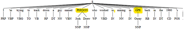
Notice that the named entities are labeled with their types of entities. For instance, Ouray is tagged with GPE, which stands for geo-political entities.

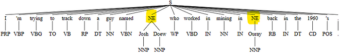
The ne_chunk() function also has a binary=True argument where, if specified, we only get the named entities labeled with NE showing that they are named entities rather than what type they are.

named_ent_txt = "I'm trying to track down a guy named Josh Doew who worked in mining in Ouray back in the 1960's."
tree = nltk.ne_chunk(nltk.pos_tag(word_tokenize(named_ent_txt)), binary=True)

tree

Rather than displaying a tree of all the named entities, we can create a function to extract them without any repeats and store them as a list.

To do so, we will need to tokenize the text, tag the words with their respective PoS and then extract the named entities based on those PoS tags without repetition if a word exists multiple times.

In the function, we loop to find the presence of the chunk structure where the chunk structure is of type Tree with tokens and chunks (subtree with tokens). In our case, these chunks are:

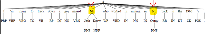
So, we need to convert them back into a list of tokens with theleaves()method and add them back into the contionus_chunk.

def extract_named_entities(text):
  tree = nltk.ne_chunk(nltk.pos_tag(word_tokenize(text)))
  continuous_chunk = []
  current_chunk = []

  for chunk in tree:
    if type(chunk) == Tree:
      current_chunk.append(" ".join([token for token, pos in chunk.leaves()]))
      if current_chunk:
        named_entity = " ".join(current_chunk)
        if named_entity not in continuous_chunk:
          continuous_chunk.append(named_entity)
          current_chunk = []
      else:
        continue
  return continuous_chunk

# call the function
extract_named_entities(named_ent_txt)

# RESULTS

['Josh Doew', 'Ouray']

Great!

Word Frequency Distribution

We can identify words frequently appearing in our text data by building a frequency distribution. To do this, we use the FreqDist module in NLTK.

Let’s use the tokens_no_stopwords list derived from removing the stop words section.

from nltk import FreqDist
freq_distribution = FreqDist(tokens_no_stopwords)

# extract the 10 frequent words in the text
freq_distribution.most_common(10)

# RESULTS

'''
[(',', 3),
 ('much', 1),
 ('natural', 1),
 ('language', 1),
 ('processing', 1),
 ('ranging', 1),
 ('speech', 1),
 ('recognition', 1),
 ('recommendation', 1),
 ('systems', 1)]

'''

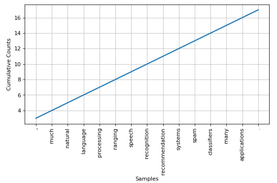
We can also visualize the distribution:

freq_distribution.plot(20, cumulative=True)

With the knowledge we have gained on text preprocessing with NLTK, it’s time to put some of it into use. Next, we will build an Email Spam Classifier.

Email spam classification with TensorFlow, Keras, and NLTK.

This section will create a spam classification model with TensorFlow and Keras. The ability to classify a text/email sent to you as spam or ham (not harmful) is a crucial functional detail in many messaging applications we use today, like Gmail or Apple’s official messaging app.

The following are the steps we will take:

• First, initialize Comet tracking
• Take care of all the necessary imports
• Grab a dataset and visualize it with Kangas.
• Preprocessing the data
  – Removing stop words.
  – Tokenizing the text data.
  – Lemmatization — We will choose Lemmatization over Stemming for the best performance of our model.
  – Vectorizing the data.
• Building the model.
• Evaluating the model.

Initialize Comet tracking

To use comet, we will need a personal API key that will be used to communicate between your experiment and the comet platform. Sign up and find the API key under your Account Settings under your profile.

Also, install comet_ml with pip, if not installed in your environment:

# on Juypyter

%pip install comet_ml

# on command line

pip install comet_ml

# initialize comet

import comet_ml

experiment = comet_ml.Experiment(
    api_key="your_API_Key", #Use your api_key from your comet_account
    project_name="Email Spam Classifier", 
    log_code=True,
    auto_metric_logging=True,
    auto_param_logging=True,
    auto_histogram_weight_logging=True,
    auto_histogram_gradient_logging=True,
    auto_histogram_activation_logging=True,
)

We are good to go!

Let’s take care of all the necessary imports:

# for data
import numpy as np
import pandas as pd

# for visuals
from matplotlib.pyplot import figure, plt
import seaborn as sns
from wordcloud import WordCloud

# from nltk for NLP
import nltk
import string # for use in punctuation removal
from nltk.corpus import stopwords
from nltk.tokenize import word_tokenize
from nltk.stem import WordNetLemmatizer

# text preprocessing from sklearn
from sklearn.feature_extraction.text import TfidfVectorizer
from sklearn.model_selection import train_test_split

# for the NN
import tensorflow as tf
from tensorflow import keras
from tensorflow.keras.models import Sequential
from keras.layers import Dense

# Evaluation
from sklearn.metrics import confusion_matrix, classification_report, accuracy_score, precision_score, recall_score, f1_score

Working on the dataset for NLP

We will use the spam collection dataset from Kaggle. We will read the data using Kangas Datagrid.read_csv() class method.

I know we are used to Pandas, but this time let’s do it the Kangas way.

Simply install Kangas with %pip install kangas on your notebook.

Reading and visualizing the data with Kangas

First, we need to import the kangas with alias kg:

import kangas as kg

# Read the data using Kangas
dg = kg.DataGrid.read_csv("spam_data.csv")
dg.save()

When we read the data with Kangas, we get a DataGrid, unlike in Pandas with DataFrame. We can perform most of the functions of Pandas, like head(), tail(), etc, with the DataGrid.

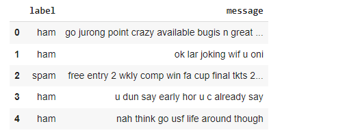
# For example get the first ten rows

dg.head(10)

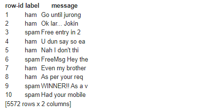
# Get the columns

dg.get_columns()

# ['label', 'message']

However, this is not the goal of Kangas. Kangas has a user interface that we can see more clearly and beautifully visualize our data. To fire up the UI, we call the show() method on the DataGrid:

#Fire up the Kangas UI

dg.show()

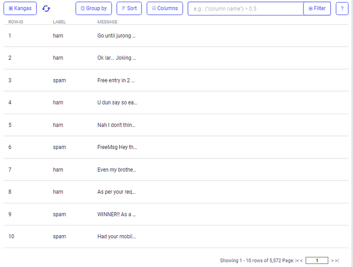
Clearly, we can visualize:

• The first ten rows of our data(dg.head(10)).
• The columns (ROW-ID, LABEL, MESSAGE)(dg.get_columns()).

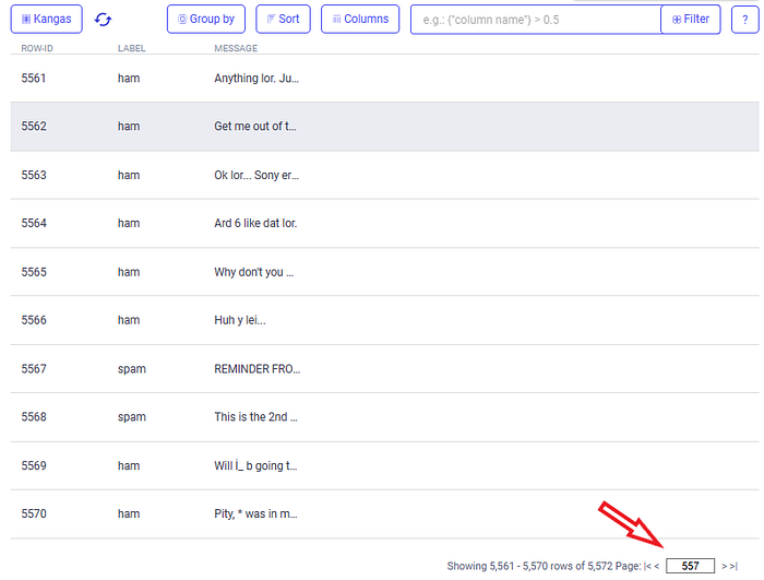
Visualize the last rows of the data(dg.tail()):

We can check the value counts of the spam and ham messages. Use Group by labels on the UI:

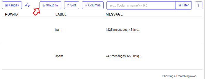
We have 4825 messages that are ham and 747 messages that are spam.

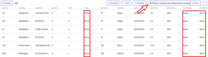
We can also check if we have null values in the data. To do this on the UI, DataGrid has filter expressions that we can use.

We use is Noneto check for null values where we will combine expressions with and and use parenthesis to force evaluation.

To check if we have null values:

# paste this on the UI's Filter input box

(({"message"} is None) and ({"label"} is None))

Since we have no matching rows for our criteria it means we have no null values.

To quench your curiosity, here is an example where we would have null values filtered from another dataset using the criteria in the UI:

It is also good that we check for empty strings. Sometimes, a database will fill with empty strings when no data is found somewhere.

empty_strs = []
for iter, label, msg in df.itertuples(name="Ham_spam"):
  if msg.isspace():
    empty_strs.append(1)

# Result is a empty list as we have no empty strings
[]

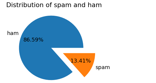
Just to be “fancy”, let’s check the percentage distribution of each label (ham and spam):

category_count = df['label'].value_counts()

fig , ax = plt.subplots(figsize=(15, 5))
explode = [0.1, 0.3]
ax.pie(category_count, labels=category_count.index, explode=explode, autopct='%1.2f%%')
ax.set_title('Distibution of spam and ham')
plt.show()

Preprocessing the text data with NLTK

Here we will:

• Tokenize each message in the message column.
• Convert all text to lowercase and remove stop words and punctuations.
• Lemmatize the message.

We have chosen to use lemmatization on the dataset since it performs better and gives meaningful words.

Let’s create a function that does the above processes for us.:

import re

def preprocess_mesg(message):

  # define list to hold all the preprocessed words
  preprocessed_msg = [] 

  # first lets convert the messages into lower case
  message_lower = message.lower()
  message = re.sub(r'[^a-zA-Z0-9\s]', ' ', message_lower)

  # combine stopwords, and punctuations
  stopword_and_punctiation = set(stopwords.words('english') + list(string.punctuation))
  
  # tokenize each message with word_tokenize
  message = word_tokenize(message)

  # Initialize the lemmatizer
  lemmatizer = WordNetLemmatizer()

  # clean the message
  cleaned_message = [preprocessed_msg.append(lemmatizer.lemmatize(word)) for word in message if word not in stopword_and_punctiation]
  cleaned_message = " ".join(preprocessed_msg)
  
  return cleaned_message

df['message'] = df['message'].apply(preprocess_mesg)

If we display the DataFrame, we get a column with cleaned messages with no stop words, lowercase, and lemmatized.

Since our data is now clean, we need to grab the predictor and the target variables.

messages = df['message'].values # X
labels = df['label'].values # y

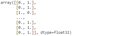
We will convert the labels into numerical types with Keras’ one-hot-encoding using to_categorical() method.

from keras.utils import to_categorical

label2int = {'ham': 1, 'spam':0}
labels = [label2int[label] for label in labels]
labels = to_categorical(labels)

labels

Splitting the data into training and test sets

We need to split and shuffle the data into training sets for training the model and test sets for evaluating the model’s performance.

X_train, X_test, y_train, y_test = train_test_split(messages, labels, test_size=0.30, random_state=42)

X_train.shape, X_test.shape, y_train.shape, y_test.shape

# Shapes
((3900,), (1672,), (3900, 2), (1672, 2))

Feature extraction with TfidfVectorizer

Before training our model, we need to convert our training samples into computer-understandable numerical data.

The common way we do this is by using the TfidfVectorizer from Scikit-learn. We could use the CounterVectorizer for this, but as the CountVectorizer only returns a sparse matrix of the only integer counts of the words, TfidfVectorizer returns only floats as scores as it takes into consideration the importance of each word. This means that less important words will have very low scores, thus helping improve our model.

# initialize the vecotrizer

tfidfV = TfidfVectorizer()

# transform the train and test sets and transform to array
X_train_tfidfV = tfidfV.fit_transform(X_train).toarray()
X_test_tfidfV = tfidfV.transform(X_test).toarray()

Building the model

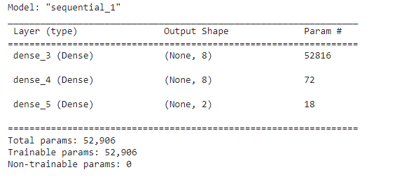
Here we will use the Keras Sequential model and set the input dimensions equal to the training data we have vectorized.

We will also use rectified linear activation function(relu) activation function for our hidden layers and the softmax function, which will convert the vectors into probability distributions for our output layer.

# initialize the Sequential model
model = Sequential()

input_dim = X_train_tfidfV.shape[1]

# add Dense layers to the neural network
model.add(Dense(8, input_dim=input_dim, activation='relu'))
model.add(Dense(8, input_dim=input_dim, activation='relu'))
model.add(Dense(2, activation='softmax'))

model.compile(loss='categorical_crossentropy', optimizer='adam', metrics='accuracy')

# call the summary method of the model

model.summary()

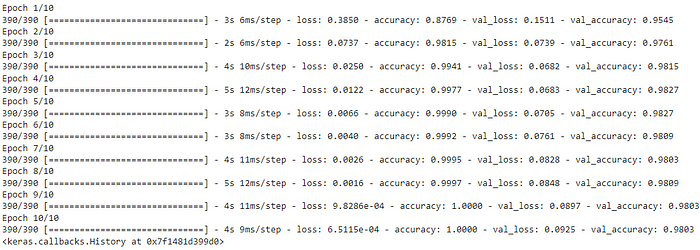
Next, we need to train the model for the fixed number of epochs or iterations on the dataset using the fit method of the Sequential model class.

We will iterate through the training set 10 times(epochs), from which we will pick the validation data before the model is trained. The validation data will help gauge the model’s performance and losses, which can help us identify if it is overfitting or not.

model.fit(X_train_tfidfV, y_train, epochs=10, verbose=True, validation_data=(X_test_tfidfV, y_test) ,batch_size=10)

Evaluating the model

Now that our model is trained, we can create the confusion matrix and classification report. We will also view the performance in Comet.

preds = (model.predict(X_test_tfidfV) > 0.5).astype("int32")

# round the testing and predictions data

y_test = np.argmax(y_test, axis=1)
preds = np.argmax(preds, axis=1)

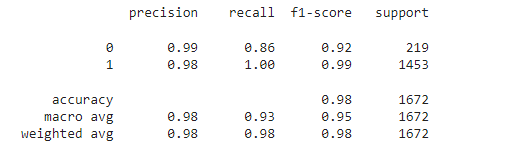
Classification report:

print(classification_report(y_test, preds))

Confusion matrix:

figure(figsize=(7, 5), dpi=80)
sns.heatmap(pd.DataFrame(cf_matrix), annot=True, cmap="YlGnBu" ,fmt='g', cbar=False)
plt.title('Confusion matrix', y=1.1)
plt.ylabel('Actual label')
plt.xlabel('Predicted label')

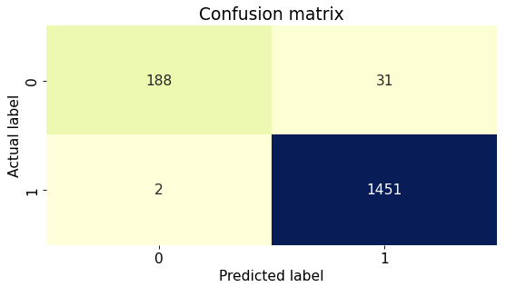
Looking at the confusion matrix, we can see that the model has high TP (188) and TN (1451) rates and low FP and FN rates. Thus, it is predicted remarkably.

Comet time!

To view the experiment on Comet, include the following line in the last cell of your notebook or code.

experiment.end()

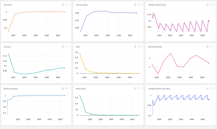
The accuracy and the loss and validation loss are logged automatically on Comet:

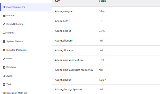
Comet will also show the hyperparameters on the trained model automatically.

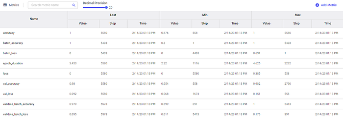
Metrics:

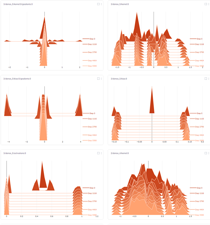
We can also view visualizations for the gradients, activations, weights, and biases. For instance, we can see the biases over each epoch in the visualizations below.

Comet is a beneficial platform for building models that entirely encourages you to focus on developing the particular model, and the rest will be logged out for you.

Final thoughts

Natural language processing is a broad field and is not limited to classifying spam in text. You can ideally use the knowledge you have gained on text preprocessing with NLTK to explore other NLP tasks.

Also, we have not exhausted all the capabilities of NLTK in text preprocessing. However, we have covered the most common concepts you will begin with when doing NLP.

This is an all-in-one article where you have learned.

• NLTK text preprocessing concepts.
• Visualizing data with Kangas.
• Vectorizing data with TFidfVectorizer. Also, explore other methods like CounterVectorizer for the same function.
• Building an email spam classifier using TensorFlow and Keras.
• Tracking your experiment with Comet and viewing the various metrics and visualizations produced by the platform.