Note: This is the part 3 of the series Major Problems of Machine Learning Datasets. You can read part 1 here and part 2 here.

Imbalanced data

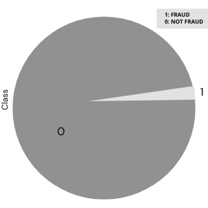
Imbalanced data occurs when there is an uneven distribution of classes or labels. For example, in a credit card detection task, the number of non-fraudulent transactions will likely be much greater than the number of fraudulent credit card transactions.

Particularly with classification tasks, class balance is extremely important. When classes are imbalanced, the majority class will influence the output of the model more, making our classifier biased towards the majority class.

Models trained with imbalanced data usually have high precision and recall scores for the majority class, whereas these scores will likely drop significantly for the minority class.

Let’s take a look at this example of a credit card fraud dataset, and build a model on this imbalanced data. Our goal is to correctly identify fraudulent transactions:

import pandas as pd
import seaborn as sns
import matplotlib.pyplot as pltdf = pd.read_csv("creditcard.csv")# checking class distribution of column `Class`
sns.countplot(data= df, x = "Class")

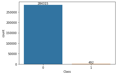
We have a clear class imbalance here. Let’s see how much this will affect model performance:

#  Splitting Data Into Training and Test Sets
from sklearn.model_selection import train_test_split
X_train, X_test, y_train, y_test = train_test_split(X,
                                                    y,
                                                    test_size=0.2,
                                                    random_state=42)
print(X_train.shape, vX_test.shape)
------------
(227845, 30) (56962, 30)

Now that the data is divided into training and test sets, let’s build a baseline logistic regression model.

from sklearn.linear_model import LogisticRegression
lr = LogisticRegression(solver='liblinear')
lr.fit(X_train, y_train)

Now we evaluate the performance of the model with a classification report and confusion matrix:

from sklearn.metrics import (plot_confusion_matrix,
                             classification_report)
def gen_report(model):
  preds = model.predict(X_test)
  print(classification_report(preds, y_test))
  plot_confusion_matrix(model, X_test, y_test)print("---LOGISTIC REGRESSION MODEL---")
gen_report(model=lr)

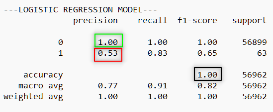
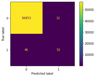
A quick look at these metrics, and it would seem our model performs amazingly — 100% accuracy, 100% precision, and 100% recall! But if we dig a little deeper, we’ll see that our precision drops to 53% on fraudulent data (the minority class) and recall drops to 83%.

How to deal with imbalanced data

The first thing we can do is change our sampling method. Instead of random sampling, we can use stratified sampling, which makes sure train and test data will have an almost equal ratio of fraudulent transactions. The downside to this method, however, is that with such a small proportion of total minority class cases in the total data, we will still have very few instances of fraudulent cases present for the model to learn from.

Instead, we might try a resampling method that attempts to tackle the underlying problem of not enough representation of the minority class. Resampling includes both oversampling and under-sampling methods.

Oversampling is a resampling technique using which generates more instances of the underrepresented class by randomly sampling from the existing instances.

Under-sampling is a resampling technique in which the majority class is reduced to the size of the minority class by randomly sampling from the majority class.

Scikit-learn’s imblearn is an open-source, MIT-licensed Python library that provides tools to deal with imbalanced classes. It has a class named SMOTETomek that combines the concepts of under-sampling and oversampling techniques, theoretically providing a good compromise between the pros and cons of each (though in practice this is not always the case; for your dataset, you may need to experiment with each sampling method to see which performs best for your dataset).

from imblearn.combine import SMOTETomek
smt = SMOTETomek()X_res, y_res= smt.fit_resample(X, y)

Let’s again create a model on our resampled data and see if performance improves:

from sklearn.model_selection import train_test_split
X_train, X_test, y_train, y_test = train_test_split(X_res,
                                                    y_res,
                                                    test_size=0.2,
                                                    stratify=y,
                                                    random_state=42
                                                    )
from sklearn.linear_model import LogisticRegression
re_lrm = LogisticRegression(solver='liblinear')
re_lrm.fit(X_train, y_train)
print("---LOGISTIC REGRESSION MODEL (RESAMPLED)---")
gen_report(model= re_lrm)

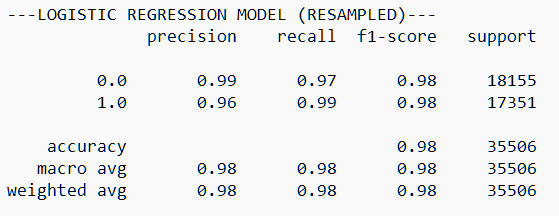
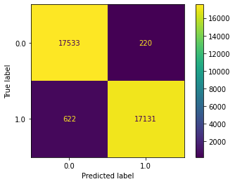
As you can see, we’ve had a vast improvement in model performance!

High-dimensional data

In machine learning, the number (or, degree) of features in a dataset is referred to as its dimensionality. Machine learning problems with high dimensionality have a variety of issues.

As the number of features in a dataset increases, the time needed to train the model will also increase. But that’s not all. High-dimensional datasets are extremely difficult (if not impossible) to visualize (imagine a 6-dimensional plot… neither can I!). The harder it is to visualize a dataset, the harder it can be to explain, which contributes to the “black box” problem in machine learning. Furthermore, the amount of data needed to train a model typically grows exponentially with the number of features (or, dimensions) in a dataset. This is often referred to as the Curse of Dimensionality and can lead to a slew of statistical phenomena that do not occur in low-dimensional settings. To save our model from this problem, we can perform dimensionality reduction.

Want to see the evolution of AI-generated art projects? Visit our public project to see time-lapses, experiment evolutions, and more!

How to deal with high dimensionality

Dimensionality reduction attempts to reduce the number of features in a dataset, while still preserving as much variation as possible from the original data. Dimensionality reduction can reduce the chances of overfitting, takes care of multicollinearity, removes noise from data, and can also be useful to transform non-linear data into linear data.

There are two main techniques to perform dimensionality reduction: we can either remove the least important feature, or we can try to combine the original features into newer, fewer features. One of the most popular methods of linear dimensionality reduction is PCA (Principle Component Analysis).

PCA transforms a set of correlated features into a smaller number of uncorrelated features, called principal components. PCA makes use of the correlation between features for reducing dimensions. Note that it is important to perform feature scaling before applying PCA because it is very sensitive to relative ranges of features.

Sci-kit learn provides a built-in tool for this process with sklearn.decomposition.PCA.

Let’s first scale the data using Standard Scaler:

from sklearn.preprocessing import StandardScalerscaler = StandardScaler()
scaler.fit(X)
X_scaled = scaler.transform(X)

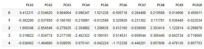
And now let’s apply PCA:

from sklearn.decomposition import PCApca_10 = PCA(n_components = 10, random_state = 42)
X_pca_10 = pca_10.fit_transform(X_scaled)# comparing before and after PCA shape
print(X.shape, X_pca_10.shape)
------------
((284807, 30), (284807, 10))

Non-normal distribution of data

The normal distribution is a type of distribution of data in which data points are distributed in a symmetrical manner around the mean of data. It looks like a bell shape curve.

It is important for most machine learning algorithms that features should follow a normal distribution. non-normal distribution of data affects model performance and generates wrong predictions normality is an important assumption for many machine learning models.

In this blog, we will discuss the two most common types of non-normal distribution Left skewed and right-skewed distribution.

The left-skewed distribution has a long tail with negatively-skewed data, whereas the right skewed has a long tail on the right side of the distribution.

How to Deal With Non-Normal Distribution of Data

There are many transformation methods that are used to convert non-normal distribution into a normal distribution.

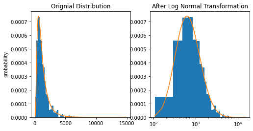
1. Log Normal Transformation: In this technique, we take the log of values of a particular feature.

import numpy as np
import matplotlib.pyplot as plt
from scipy import stats# sample data generation
np.random.seed(42)
data = sorted(stats.lognorm.rvs(s=0.5, 
                                loc=1, 
                                scale=1000, 
                                size=1000))# fit lognormal distribution
shape, loc, scale = stats.lognorm.fit(data, loc=0)
pdf_lognorm = stats.lognorm.pdf(data, shape, loc, scale)

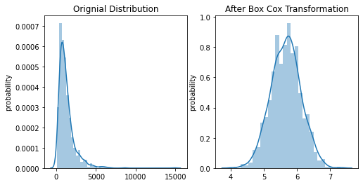
2. Box-Cox Transformation: Box-Cox transformation is a part of the power transformers family. It makes use of the exponent lambda (λ), which ranges from -5 to 5, to convert non-normal distribution of dependent variables into a normal distribution.

import numpy as np
import matplotlib.pyplot as plt
from scipy import stats# sample data generation
np.random.seed(42)
data = sorted(stats.lognorm.rvs(s=0.7, loc=3, scale=1000, size=1000))pdf_boxcox = stats.boxcox(data)