Data play a key role in machine learning, and the better and more relevant data you have, the more accurate the model you will build. Getting the perfect data, however, is still a dream for many data scientists. A lot of data comes from web scraping, APIs and other external sources, and most real-world datasets will just look like an ugly stack of information, at least at first. However, data will speak for itself, if you keep it organized.

In this blog, I would love to share some major problems that occur with many supervised machine learning datasets, as well as how to deal with them.

Missing Values

How to Deal with Missing Values In Datasets?

There are various ways of dealing with missing values, and you’ll likely need to determine which method is right for your task at hand on a case-by-case basis. If only a very small percentage of your data is missing, then you might be able to simply drop all missing values. In some cases of extremely large amounts of missing data, it may even be better to consider finding a new dataset, additional datasets, increasing your domain knowledge, or reframing your problem. When about 10–50% of your data are missing, however, you may also consider imputation.

There are two types of imputation: numerical and categorical.

Imputing Missing Numerical Data

1. Mean, median, or mode imputation: If the distribution of your data appears normal, you might consider calculating the mean of a particular feature to replace missing values. However, if the distribution of data appears left- or right-skewed, then you might be better off with median imputation. The following implementation assumes that your missing values are represented by NaNs:

# import numpy as np# Normally-distributed data (fill with mean)
df['col'] = df['col'].fillna(df['col'].mean()) # Skewed data (fill with median)
df['col'] = df['col'].fillna(df['col'].median())

2. Treat NaN as new category: This technique is useful when there is some relationship between missing values and non-missing values. In this method, we add a new column to our DataFrame with all missing values as 1 and non-missing values as 0. Note that this method creates a category feature out of whether or not a missing value exists in a particular numerical feater, but does not replace, or otherwise handle, the original missing values. Later we should still replace missing values from the original column.

import numpy as npdf['col_nan']= np.where(df['col'].isnull(),1,0) df['col'] = df['col'].fillna(df['col'].mean()) 

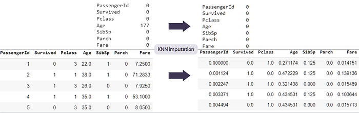
3. KNN Imputer: KNN Imputer is a distance-based imputation method that utilizes the k-Nearest Neighbors algorithm to replace missing values in the dataset with the mean value of k nearest neighbors found in training data. The value of k is determined using the parameter n_neighbors. By default, KNN uses the Euclidean distance metric to find the nearest neighbors. One thing to remember is that we need to normalize the data before passing it to KNN Imputer, otherwise replacements will be biased towards the larger range of features.

# Loading DataFrame
import pandas as pd
df = pd.read_csv('titanic.csv')# Extracting all Columns With Numerical Data
num = [col for col in df.columns if df[col].dtypes != 'O']# Scaling Data Using MinMaxScaler
from sklearn.preprocessing import MinMaxScaler
scaler = MinMaxScaler()
norm_df = pd.DataFrame(scaler.fit_transform(df[num]), columns = num)# Initialize Imputer
from sklearn.impute import KNNImputer
knn = KNNImputer(n_neighbors=5)# Fit Imputer and Transform Data
knn.fit(norm_df)# Transform Data and Save It In a New Instance of DataFrame
non_nan_df=pd.DataFrame(knn.transform(norm_df), columns=num)

This method can also be used for categorical data, but for that, we first need to convert the data to numerical form using label- or one-hot-encoding.

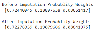
4. Filling categories proportionally using their probability weights: In this technique, we replace missing categories with other categories based on their contribution to creating the whole feature. This method doesn’t change the category proportion, which means In a feature if category A contributes 90%, B 7%, and C 3% then after filling missing values proportion of A, B and C will stay almost the same.

def fill_proportionally(col, dataset):
    import random
    random.seed(0)
    
    # getting all unique values (without nan)
    values = dataset[col].dropna().unique()
    
    # getting weights for probability weighting
    weights = dataset[col].value_counts().values / dataset[col].value_counts().values.sum()
    print('Before Imputation Probablity Weights\n',weights)
    # filling
    dataset[col] = dataset[col].apply(lambda x: random.choices(values, weights=weights)[0] if pd.isnull(x) else x)
    
import pandas as pd
df = pd.read_csv('https://raw.githubusercontent.com/Abhayparashar31/datasets/master/titanic.csv')

### Imputing Missing Categories 
fill_proportionally('Embarked', df)

There are other methods as well that make use of machine learning models to predict missing values. You can check them by visiting my Kaggle notebook.

Innovation and academia go hand-in-hand. Listen to our own CEO Gideon Mendels chat with the Stanford MLSys Seminar Series team about the future of MLOps and give the Comet platform a try for free!

Categorical Data

Many machine learning algorithms work only with numerical data including regression models. For this reason, it is important to convert categorical data to a numerical form before feeding them to a machine learning model. Categorical data refer to data with labels as values (e.g., sex, city, position, etc.).

How to deal with categorical data in datasets?

One option when utilizing categorical data is to choose a tree-based model, when appropriate. If the situation calls for another type of model, however,
then another option is to convert the categorical values into numerical form.

Imputing Categorical Data (with no inherent order)

Inherent order means there is a relationship between the order of our categories. In categories with no inherent order, we can use nominal encoding methods. One of the most common methods of nominal encoding is One-Hot Encoding

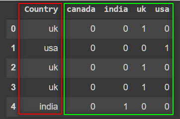
• One-Hot Encoding: In One-Hot encoding, we create new columns to represent each individual class label, and ascribe 0 or 1 values to each feature, depending on whether or not they belong to a particular class. This approach can be used for both single- and multi-class categorical values. One major downfall of this method, however, is that increases the dimension of the data.

import pandas as pd
import numpy as np

### Sample Data Creation
countries = ['india','uk','usa','canada']
col = np.random.choice(countries,100)
df = pd.DataFrame(col,columns=['Country'])

### One Hot Encoding
dummies = pd.get_dummies(df['Country'])
pd.concat([df,dummies],axis=1).head()

Imputing Categorical Data (with inherent order)

If there is some relation between the order of categories, we refer to the categories as ordinal. For these situations, we can use methods like label encoding, and target-guided encoding.

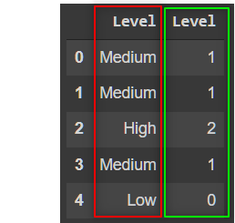
• Label Encoding: Label encoding refers to the process of converting labels into a range of numbers (not just 0 and 1), thereby preserving some of their ordinality. The major downfall of label-encoding, however, is that machines don’t just infer the order of the categories, but also the values of the numbers themselves, sometimes giving higher weight or importance to features assigned to larger category numbers.

import pandas as pd
import numpy as np

### Sample Data Creation
countries = ['Low','Medium','High']
col = np.random.choice(countries,100)
df = pd.DataFrame(col,columns=['Level'])

### Label Encoding (Sklearn)
from sklearn.preprocessing import LabelEncoder
le = LabelEncoder()
le.fit_transform(df['Level'])

### Label Encoding (Manual Method)
df['Level'].map({
    'High':2,
    'Medium':1,
    'Low':0
})

• Count Encoding: Count encoding is a simple method in which we replace all the categories with their count:

Cat_Count = df['col'].value_counts().to_dict()
df['col'].map(Cat_Count)

Different ranges

Datasets often include multiple features, each with a unique range of values. For example, a dataset containing information about salaries of different employees based on age and years of experience will have a much different range in the salary values than it will in the age values. Due to this difference, the features with higher value ranges may influence the output more.

One way to overcome this quirk is to use tree-based models like Random Forest. However, if your problem requires the use of regularized linear models or neural networks, then your should scale your feature ranges (e.g., 0 to 1).

Feature scaling techniques:

1. Min Max Scaler: By default, this method scales all data between 0 and 1. However, you can also use a min-max scaler to scale values within a custom range.

from sklearn.preprocessing import MinMaxScaler# Defining Scaler
scaler = MinMaxScaler()# Scaling Columns Values
column_names = ['salary_col', 'age_col']
features = df[column_names]
features[column_names] = scaler.fit_transform(features.values)

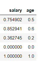
You can change the scaling range by specifying feature_range = (lower, upper).

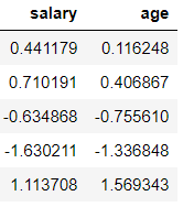
2. Standard Scaler: This method assumes that values of the column are normally distributed. It scales values in a way that the mean of all the values is 0 and the standard deviation is 1.

from sklearn.preprocessing import StandardScaler# Defining Scaler
scaler = StandardScaler()col_names = ['salary', 'age']
features = df[col_names]# Scaling Values
features[col_names] = scaler.fit_transform(features.values)
features

There are other scalers as well that are somewhat less famous, but still useful, including: Robust Scaler, MaxAbsScaler, Quantile Transformer Scaler, and many more. You can learn about all of them by reading my previous article about feature scaling and transformation.

Too little training data

Too little training data is a major problem for computer vision datasets, a popular section of deep learning. These models require incredibly large amounts of labeled training data, which tends to be expensive to produce, and limited in availability. The simple and straightforward approach would be to collect more data, but in reality, this is not possible every time. Instead, we’ll often use data augmentation.

Image data augmentation

Image data augmentation is a technique in which we apply certain transformations to existing image data in order to generate multiple, unique copies for training purposes. Some transformations include rotating, cropping, padding, scaling, flipping, changing brightness, adding noise, and many more.

We can perform image augmentation manually using python, pillow, and OpenCV library. One automated way of doing this uses the deep learning library Keras. In the Keras image class, is the ImageDataGenerator method that provides different options to perform position and color augmentation.

from keras.preprocessing.image import ImageDataGenerator, array_to_img, img_to_array, load_img

datagen = ImageDataGenerator(
        rotation_range=40,
        width_shift_range=0.2,
        height_shift_range=0.2,
        brightness_range= [0.5, 1.5],
        rescale=1./255,
        shear_range=0.2,
        zoom_range=0.4,
        horizontal_flip=True,
        fill_mode='nearest',
        zca_epsilon=True)

path = '/content/drive/MyDrive/cat.jpg' ## Image Path
img = load_img(f"{path}")
x = img_to_array(img)
x = x.reshape((1,) + x.shape)
i = 0

### Create 25 Augmentated Images and Save Them In `aug_img` directory
for batch in datagen.flow(x, batch_size=1,
                      save_to_dir="/content/drive/MyDrive/aug_imgs", save_prefix='img', save_format='jpeg'):
    i += 1
    if i > 25:   ## Total 25 Augmented Images
        break

Different representations of data

1. Range instead of singular integer value

import pandas as pddf = pd.DataFrame(['10-12','15-17','20-23','18-25','26-28'],columns=['Age'])

• Replace with lower limit:

df['Age'].apply(lambda x : x.split('-')[0])

• Replace with upper limit:

df['Age'].apply(lambda x : x.split('-')[1])

• Mean of range:

import numpy as np
np.mean(lower_limit,upper_limit)

• Random value imputation from range

import random
random.randint(lower_limit,upper_limit)

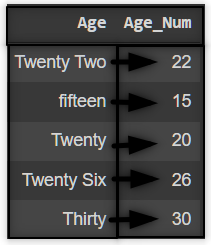
2. Conversion using numerizer

import pandas as pddf = pd.DataFrame(['Twenty Two','fifteen','Twenty','Twenty Six','Thirty'],columns=['Age'])

In the case of text or categorical representation of numerical data, we can use the numerizer library to quickly and simply transform our data:

from numerizer import numerize
df['Age'].apply(lambda x: numerize(x))

Read more in Major Problems of Machine Learning Datasets: Part 2 andMajor Problems of Machine Learning Datasets: Part 3!