A Step-by-Step Guide: Efficiently Managing TensorFlow/Keras Model Development with Comet

Welcome to the step-by-step guide on efficiently managing TensorFlow/Keras model development with Comet. TensorFlow and Keras have emerged as powerful frameworks for building and training deep learning models. However, as your model development process becomes more complex and involves numerous experiments and iterations, keeping track of your progress, managing experiments, and collaborating effectively with team members becomes increasingly challenging.

This is where Comet comes to the rescue. Comet is a comprehensive experiment tracking and collaboration platform for machine learning projects. It empowers data scientists and machine learning practitioners to streamline their model development workflow, maintain a structured record of experiments, and foster seamless collaboration among team members.

In this guide, we will walk you through the process of efficiently managing TensorFlow/Keras model development using Comet. We will explore the essential features of Comet that enable you to track experiments, log hyperparameters and metrics, visualize model performance, optimize hyperparameter configurations, and facilitate collaboration within your team. Following our step-by-step instructions and incorporating Comet into your workflow can enhance productivity, maintain experiment reproducibility, and derive valuable insights from your model development process.

Whether you are an experienced machine learning practitioner or just starting your journey in deep learning, this article will provide practical strategies and tips to leverage Comet effectively. Let’s dive in and discover how you can take control of your TensorFlow/Keras model development with Comet.

Introducing MLOps

Machine learning (ML) is an essential tool for businesses of all sizes. However, deploying ML models in production can be complex and challenging. This is where MLOps comes in.

MLOps is a set of principles and practices that combine software engineering, data science, and DevOps to ensure that ML models are deployed and managed effectively in production. MLOps encompasses the entire ML lifecycle, from data preparation to model deployment and monitoring.

Why Is MLOps Important?

There are several reasons why MLOps is essential. First, ML models are becoming increasingly complex and require a lot of data to train. This means it is necessary to have a scalable and efficient way to deploy and manage ML models in production.

Second, ML models are constantly evolving. This means that it is vital to have a way to monitor and update ML models as new data becomes available. MLOps provides a framework for doing this.

Finally, ML models need to be secure. They can make important decisions, such as approving loans or predicting customer behavior. MLOps provides a framework for securing ML models.

How Does MLOps Work?

MLOps typically involves the following steps:

1. Data Preparation: The first step is preparing the data that will be used to train the ML model. This includes cleaning the data, removing outliers, and transforming the data into a format that the ML model can use.
2. Model Training: The next step is training the ML model. This involves using the prepared data to train the model. The training process can be iterative, and trying different models and hyperparameters may be necessary to find the best model.
3. Model Deployment: Once the ML model is trained, it must be deployed in production. This means making the model available to users so they can use it to make predictions.
4. Model Monitoring: Once the ML model is deployed, it must be monitored to ensure it performs as expected. This involves tracking the model’s accuracy, latency, and other metrics.
5. Model Maintenance: As new data becomes available, the ML model may need to be updated. This is known as model maintenance. Model maintenance involves retraining the model with the latest data and deploying the updated model in production.

Keeping Track of Your ML Experiments

Accurate experiment tracking simplifies comparing metrics and parameters across different data versions, evaluating experiment results, and identifying the best or worst predictions on test or validation sets. Additionally, it allows for in-depth analysis of hardware consumption during model training.

The following explanations will guide you in efficiently tracking your experiments and generating insightful charts. By implementing these strategies, you can enhance your experiment management and visualization capabilities, allowing you to derive valuable insights from your data.

Project Requirements

To ensure adequate tracking and management of your TensorFlow model development, it is crucial to establish a performance metric as a project goal. For instance, you may set the F1-score as the metric to optimize your model’s performance.

The initial deployment phase should focus on building a simple model while prioritizing the development of a robust machine-learning pipeline for prediction. This approach allows for the swift delivery of value and prevents excessive time spent pursuing the elusive perfect model.

As your organization embarks on new machine learning projects, the number of experiment runs can quickly multiply, ranging from tens to hundreds or even thousands. Without proper tracking, your workflow can become convoluted and challenging to navigate.

That’s why tracking tools like Comet have become standard in machine learning projects. Comet enables you to log essential information such as data, model architecture, hyperparameters, confusion matrices, graphs, etc. Integrating a tool like Comet into your workflow or code is relatively simple compared to the complications that arise when you neglect proper tracking.

To illustrate the tracking approach, let’s consider an example where we train a text classification model using TensorFlow and Long Short-Term Memory (LSTM) networks. Following the steps in this guide will provide insights into effectively utilizing tracking tools and seamlessly managing your TensorFlow/Keras model development process.

Achieve a Well-Organized Model Development Process with Comet

Install Dependencies For This Project

We’ll be using Comet in Google Colab, so we need to install Comet on our machine. Follow the commands below to do this.

`%pip install comet_ml tensorflow numpy
  !pip3 install comet_ml
   import comet_ml
   from comet_ml import Experiment
   import logging

logging.basicConfig(level=logging.INFO)
LOGGER = logging.getLogger("comet_ml")

Now that we’ve installed the necessary dependencies let’s import them.

import comet_ml
from comet_ml import Experiment
import logging
import pandas as pd
import tensorflow as tfl
import numpy as np
import csv
from tensorflow.keras.preprocessing.text import Tokenizer
from tensorflow.keras.preprocessing.sequence import pad_sequences
from tensorflow import keras
from tensorflow.keras import layers
import re
import nltk

nltk.download('stopwords')
from nltk.corpus import stopwords

Connect your project to the Comet platform. If you’re new to the platform, read the guide.

`# Create an experiment
experiment = comet_ml.Experiment(
    project_name="Tensorflow_Classification",
    workspace="olujerry",
      api_key="YOUR API-KEYS",
    log_code=True,

   auto_metric_logging=True,
    auto_param_logging=True,
    auto_histogram_weight_logging=True,
    auto_histogram_gradient_logging=True,
    auto_histogram_activation_logging=True,

It’s important to connect your project to the Comet platform at the beginning of your project so every single parameter and metric can be logged.

Save the Hyperparameters (For Each Iteration)

params={
                    'embed_dims': 64,
                    'vocab_size': 5200,
                    'max_len': 200,
                    'padding_type': 'post',
                    'trunc_type': 'post',
                    'oov_tok': '<OOV>',
                    'training_portion': 0.75
    }

experiment.log_parameters(params)

About The Dataset

The dataset we’re using is BBC news article data for classification. It consists of 2225 documents from the BBC News website corresponding to stories in five topical areas from 2004–2005.

• Class Labels: 5 (business, entertainment, politics, sport, tech)
• Download the data here.

In the below section, I’ve created a list called labels and text, which will help us store the labels of the news article and the actual text associated with it. We’re also removing the stopwords using nltk.

labels = []
texts = []

with open('dataset.csv', 'r') as file:
    data = csv.reader(file, delimiter=',')
    next(data)
    for row in data:
        labels.append(row[0])
        text = row[1]
        for word in stopwords_list:  # Iterate over the stop words list
            token = ' ' + word + ' '
            text = text.replace(token, ' ')
            text = text.replace(' ', ' ')
        texts.append(text)

print(len(labels))
print(len(texts))

Let’s split the data into training and validation sets. If you look at the above parameters, we’re using 80% for training and 20% for validating the model we’ve built for this use case.

`training_portion = 0.8  # Assigning a value of 0.8 for an 80% training portion
train_size = int(len(texts) * training_portion)

train_text = texts[0:train_size]
train_labels = labels[0:train_size]

validation_text = texts[train_size:]
validation_labels = labels[train_size:]

To tokenize the sentences into subword tokens, we will consider the top five thousand most common words. We will use the “oov_token” placeholder when encountering unseen special values. For words not found in the “word_index,” we will use “<00V>”. The “fit_on_texts” method will update the internal vocabulary utilizing a list of texts. This approach allows us to create a vocabulary index based on word frequency.

`vocab_size = 10000  # Assigning a value for the vocabulary size
 oov_tok = '<OOV>'  # Assigning a value for the out-of-vocabulary token
tokenizer = Tokenizer(num_words = vocab_size, oov_token=oov_tok)
tokenizer.fit_on_texts(train_text)
word_index = tokenizer.word_index
dict(list(word_index.items())[0:8])

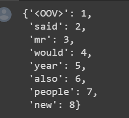
Observing the provided output, we notice that “<oov>” is the most frequently occurring token in the corpus, followed by other words.

With the vocabulary index constructed based on frequency, our next step is converting these tokens into sequence lists. The “text_to_sequence” function accomplishes this task by transforming the text into a sequence of integers. It maps the words in the text to their corresponding integer values according to the word_index dictionary.

`train_sequences = tokenizer.texts_to_sequences(train_text)
 print(train_sequences[16])
max_length = 100  # Assigning a value for the maximum sequence length

train_sequences = tokenizer.texts_to_sequences(train_text)
train_padded = pad_sequences(train_sequences, maxlen=max_length, truncating='post', padding='post')

When training neural networks for downstream natural language processing (NLP) tasks, ensuring that the input sequences are the same size is important. We can use the max_len parameter to add padding to the sequences to achieve this. In our case, we initially set max_len to 200, and we applied padding using padding_sequences.

For sequences with lengths smaller or greater than max_len, we truncate or pad them to the specified length of 200. For example, if a sequence has a length of 186, we add 14 zeros at the end to pad it to 200. Typically, we fit the data once but perform sequence conversion multiple times, so we have separate training and validation sets instead of combining them.

`padding_type = 'post'  # Assigning a value for the padding type ('post' or 'pre')


trunc_type = 'post'  # Assigning a value for the truncation type ('post' or 'pre')


valdn_padded = pad_sequences(valdn_sequences, maxlen=max_len, padding=padding_type, truncating=trunc_type)


vmax_len = 100  # Assigning a value for the maximum sequence length

valdn_sequences = tokenizer.texts_to_sequences(validation_text)
valdn_padded = pad_sequences(valdn_sequences, maxlen=max_len, padding=padding_type, truncating=trunc_type)

print(len(valdn_sequences))
print(valdn_padded.shape)

Next, let’s examine the labels for our dataset. To work with the labels effectively, we need to tokenize them. Additionally, all training labels are expected to be in the form of a NumPy array. We can use the following code snippet to convert our labels into a NumPy array.

`label_tokenizer = Tokenizer()
label_tokenizer.fit_on_texts(labels)

Before we proceed with the modeling task, let’s examine how the texts appear after padding and tokenization. It is important to note that some words may be represented as “<oov>” (out of vocabulary) because they are not included in the vocabulary size specified at the beginning of our code. This is a common occurrence when dealing with limited vocabulary sizes.

`word_index_reverse = {index: word for word, index in word_index.items()}

# %% In [41]:
def decode_article(text):
    return ' '.join([word_index_reverse.get(i, '?') for i in text])
print(decode_article(train_padded[24]))
print('**********')
print(train_text[24])

To train our TensorFlow model, we will use the tfl.keras.Sequential class that allows us to group a linear stack of layers into a TensorFlow Keras model. The first layer in our model is the embedding layer, which stores a vector representation for each word. It converts sequences of words into sequences of vectors. Word embeddings are commonly used in NLP to ensure that words with similar meanings have similar vector representations.

We then use the tfl.keras.layers.Bidirectional wrapper to create a bidirectional LSTM layer. This layer helps propagate inputs forward and backward through the LSTM layers, enabling the network to learn long-term dependencies more effectively. After that, we form it into a dense neural network for classification.

Our model uses the ‘relu’ activation function, which returns the input value for positive values and 0 for negative values. The embed_dims variable represents the dimensionality of the embedding vectors and can be adjusted based on your specific needs.

The final layer in our model is a dense layer with six units, followed by the ‘softmax’ activation function. The ‘softmax’ function normalizes the network’s output, producing a probability distribution over the predicted output classes.

Here’s the code for the model:

`embed_dims = 100  # Placeholder value, adjust it based on your needs

model = tfl.keras.Sequential([
    tfl.keras.layers.Embedding(vocab_size, embed_dims),
    tfl.keras.layers.Bidirectional(tfl.keras.layers.LSTM(embed_dims)),
    tfl.keras.layers.Dense(embed_dims, activation='relu'),
    tfl.keras.layers.Dense(6, activation='softmax')
])
model.summary()

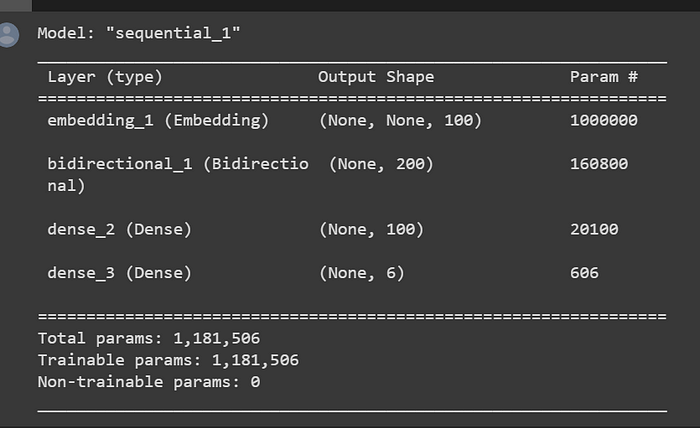
From the model summary above, we can observe that our model consists of an embedding layer and a bidirectional LSTM layer. The output size from the bidirectional layer is twice the size we specified for the LSTM layer, as it considers both forward and backward information.

We used the ‘categorical_crossentropy’ loss function for this multi-class classification task. This loss function is commonly used in tasks where we have multiple classes and want to quantify the difference between the predicted probability distribution and the true distribution.

The optimizer we have chosen is ‘adam,’ a variant of gradient descent. ‘Adam’ is known for its adaptive learning rate and performs well in many scenarios.

Our model is designed to learn word embeddings through the embedding layer, capture long-term dependencies with the bidirectional LSTM layer, and produce predictions using the softmax activation function in the final dense layer.

`model.compile(loss='sparse_categorical_crossentropy', optimizer='adam', metrics=['accuracy'])

ML Model Development Organized Using Comet

`epochs_count = 10

history = model.fit(train_padded, training_label_seq,
                    epochs=epochs_count,
                    validation_data=(valdn_padded, validation_labels_seq),
                    verbose=2)

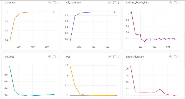
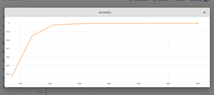
The accuracy of the experiment was logged:

We can also see the loss of the experiment:

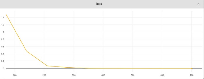
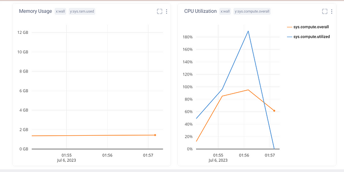
We can also monitor RAM and CPU usage as part of model training. The information can be found in the System Metrics section of the experiments.

Viewing Your Experiment On The Comet Platform

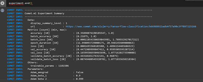
To view all your logged experiments, you need to end the experiment using the code below:

experiment.end()

After running the code, you will get a link to the Comet platform and a summary of everything logged.

Conclusion

If the above model shows signs of overfitting after 6 epochs, it is recommended to adjust the number of epochs and retrain the model. By experimenting with different numbers of epochs, you can find the optimal point where the model achieves good performance without overfitting.

Debugging and analyzing the model’s performance during development iteratively is crucial. Error analysis helps identify areas where the model may be failing and provides insights for improvement. Tracking how the model’s performance scales as training data increases is also essential. This can help determine if collecting more data will lead to better results.

Model-specific optimization techniques can be applied when addressing underfitting, characterized by high bias and low variance. This includes performing error analysis, increasing model capacity, tuning hyperparameters, and adding new features to capture more patterns in the data.

On the other hand, when dealing with overfitting, which is characterized by low bias and high variance, it is recommended to consider the following approaches:

1. Adding more training data: Increasing the training data can help the model generalize better and reduce overfitting.
2. Regularization: Techniques like L1 or L2 regularization, dropout, or early stopping can prevent the model from over-relying on specific features or reducing complex interactions between neurons.
3. Error Analysis: Analyzing the model’s errors in training and validation data can provide insights into specific patterns or classes that the model struggles with. This information can guide further improvements.
4. Hyperparameter Tuning: Adjusting hyperparameters like learning rate, batch size, or optimizer settings can help find a better balance between underfitting and overfitting.
5. Reducing Model Size: If the model is too complex, it may have a higher tendency to overfit. Consider reducing the model’s size by decreasing the number of layers or reducing the number of units in each layer.

It is also valuable to consult existing literature and seek guidance from domain experts or colleagues who have experience with similar problems. Their insights can provide helpful directions for addressing overfitting effectively.

Remember that model development is an iterative process that may require multiple iterations of adjustments and experimentation to achieve the best performance for your specific problem.

Here is a link to my notebook on Google Colab, as well as the original notebook by Aravind CR.