Computer Vision (CV) is a rapidly growing field that is transforming the way we interact with technology. As more and more companies adopt computer vision models for various applications, it has become increasingly important to monitor the performance of these models over time to ensure they continue to deliver accurate results.

In this article, we’ll introduce you to the basics of monitoring your CV models using Kangas and Comet, two powerful tools that make it easy to track and analyze the performance of your models. Whether you’re new to computer vision or have some experience under your belt, this beginner’s guide will help you gain a better understanding of the importance of monitoring your models and how to get started with these powerful monitoring tools.

We’ll cover everything from setting up your environment to tracking key metrics and analyzing the results. By the end of this article, you’ll have a solid understanding of how to monitor your CV models using Kangas and Comet, and be well on your way to delivering more accurate and reliable results.

About Comet

Comet is a powerful tool for monitoring and analyzing machine learning experiments. It allows users to track their experiments in real time, visualize the results, and share their findings with others. With Comet, users can quickly identify issues with their models, optimize performance, and collaborate with team members. It’s particularly useful for CV models, where accuracy and performance are critical to success.

About Kangas

Kangas is a robust platform for monitoring and analyzing structured and unstructured data. By using Kangas and Comet together, users can get a complete picture of their models’ performance, identify issues quickly, and collaborate with team members to optimize results.

How to Use Kangas and Comet Together

Using Kangas and Comet together provides users with a complete picture of their models’ performance. By tracking key metrics and visualizing the results, users can quickly identify issues that may impact accuracy and optimize performance over time.

To get started, you’ll need to set up your environment. Then, you can start tracking metrics and visualizing the results using the intuitive user interfaces of both tools. This makes it easy to identify trends and patterns that may impact performance, and collaborate with team members to optimize results.

The most important thing to keep in mind when building and deploying your model? Understanding your end-goal. Read our interview with ML experts from Stanford, Google, and HuggingFace to learn more.

About The Dataset

Today, we’re using the bean dataset, which is a collection of pictures of beans that were captured outdoors with smartphones. It has three classes: two for diseases and one for healthy bean plants. In this blog, we’ll attempt to differentiate between healthy and unhealthy bean leaves. You can get the data here.

Getting Started

The first step is to install all the needed libraries.

!pip3 install comet_ml --q
from comet_ml import Experiment

comet_ml.init(api_key= "YOUR-COMET-API-KEY",
              project_name= "my-project")
experiment = comet_ml.Experiment()

!pip install kangas torch datasets transformers scikit-learn --q
import kangas as kg
import tensorflow as tf
import matplotlib.pyplot as plt 
import numpy as np
from tqdm import tqdm
from tensorflow import keras
from tensorflow.keras import datasets, layers, models
from datasets import load_dataset

Next we load the dataset:

dataset = load_dataset("beans", split="train")

We then instantiate a Kangas DataGrid using our dataset:

dg = kg.DataGrid(dataset)

To show what’s in our DataGrid, we use the .show() method:

dg.show()

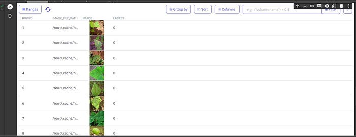
Once the dataset is loaded, we begin to investigate its filtering and group-by capabilities. In particular, we examine the bean leaf images to identify any discernible differences. We observe that the leaves labeled 0 and 1 exhibit signs of disease, while the leaves labeled 2 appear to be healthy.

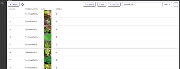
The photographs are then organized into each label using the “group-by” feature of the Kangas UI.

We then go to building the ML model so we can track using Comet.

df = pd.DataFrame(dataset)
selected_columns = df.columns[:100] # Select the first 100 columns
df = df[selected_columns] # Subset the dataframe to include only the selected columns
y_train = y_train.reshape(-1)
y_train[:5]

In the above code block, y_train = y_train.reshape(-1) reshapes the array y_train to a one-dimensional array.

The second line of code y_train[:5] selects the first five elements of the newly reshaped y_train array and returns them.

We then divide the beans dataset into classes.

classes = [ 'angular leaf spot', 'bean rust', 'healthy']

The code below defines a function called plot_sample that takes three arguments: a numpy array containing image data samples X, a numpy array containing labels for each sample in y, and an integer index index indicating which sample to plot. The function converts the index to an integer, rounds it, and creates a new figure with dimensions 15×2. It then displays the image corresponding to the selected sample and sets the x-axis label to the class label of the selected sample. The class labels are obtained from a dictionary called classes.

def plot_sample(X, y, index):
    index = np.round(index).astype(int)
    plt.figure(figsize = (15,2))
    plt.imshow(X[index])
    plt.xlabel(classes[y[index]])

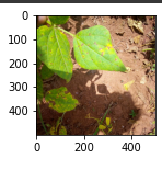
After viewing the various categories of leaves we then start building our ML model.

from tensorflow import keras
from tensorflow.keras import layers

model = keras.Sequential([
    layers.Conv2D(filters=32, kernel_size=(3, 3), activation='relu', input_shape=(500, 500, 3)),
    layers.MaxPooling2D((2, 2)),
    
    layers.Conv2D(filters=64, kernel_size=(3, 3), activation='relu'),
    layers.MaxPooling2D((2, 2)),
    
    layers.Conv2D(filters=128, kernel_size=(3, 3), activation='relu'),
    layers.MaxPooling2D((2, 2)),
    
    layers.Flatten(),
    layers.Dense(256, activation='relu'),
    layers.Dense(3, activation='softmax')
])from tensorflow import keras
from tensorflow.keras import layers

model = keras.Sequential([
    layers.Conv2D(filters=32, kernel_size=(3, 3), activation='relu', input_shape=(500, 500, 3)),
    layers.MaxPooling2D((2, 2)),
    
    layers.Conv2D(filters=64, kernel_size=(3, 3), activation='relu'),
    layers.MaxPooling2D((2, 2)),
    
    layers.Conv2D(filters=128, kernel_size=(3, 3), activation='relu'),
    layers.MaxPooling2D((2, 2)),
    
    layers.Flatten(),
    layers.Dense(256, activation='relu'),
    layers.Dense(3, activation='softmax')
])

To extract important features from input images, the model starts with a convolutional layer that uses 32 filters of size 3×3. ReLU activation function is used to deal with non-linearity. The input shape is set to (500, 500, 3), which indicates that the input image is 500×500 pixels with 3 color channels.

To reduce the input image size, a max pooling layer with a pool size of 2×2 is added to the model.

This process is then repeated two more times, with 64 and 128 filters in each convolutional layer. A max pooling layer with a pool size of 2×2 is added after each convolutional layer.

The output from the convolutional layers is then converted into a 1D feature vector using a flatten layer. Then, two fully connected layers (Dense) are added to the model, with the first layer having 256 nodes and the second layer having 3 nodes. ReLU activation function is used for the first dense layer, and softmax activation function is used for the last layer.

In multi-class classification problems, the softmax function helps normalize the output and gives a probability distribution across all classes.

The next step involves compiling the model. This is where the network architecture is configured, and the learning process is initialized with parameters such as the loss function, optimizer, and performance metrics.

model.compile(loss='categorical_crossentropy',
              optimizer='adam',
              metrics=['accuracy'])

The above code is a crucial step in configuring a neural network model for training and evaluation. It specifies the loss function, optimizer, and performance metrics that will be used during the learning process, and helps to ensure that the model is optimized for the specific problem at hand.

from datasets import load_dataset
from tensorflow.keras.utils import to_categorical

# Load the "beans" dataset
dataset = load_dataset("beans", split="train[:80%]")
val_dataset = load_dataset("beans", split="train[80%:]")

# Convert the input images to NumPy arrays
X_train = np.array([np.array(image) for image in dataset['image']])
X_val = np.array([np.array(image) for image in val_dataset['image']])

# Convert the target labels to NumPy arrays and one-hot encode them
y_train = to_categorical(np.array(dataset['labels']))
y_val = to_categorical(np.array(val_dataset['labels']))

# Compile the model
model.compile(loss='categorical_crossentropy',
              optimizer='adam',
              metrics=['accuracy'])

# Train the model
history = model.fit(X_train, y_train, batch_size=32, epochs=10, validation_data=(X_val, y_val))

The above code loads the dataset, splits it into training and validation data, converts the input images and target labels to NumPy arrays, compiles the model with the chosen optimizer, loss function, and metrics, and finally trains the model using the training data and validates it on the validation data. The training process is saved to the ‘history’ variable. This code demonstrates how to train a machine learning model on the “beans” dataset using the Keras library. It loads the dataset, splits it into training and validation data, converts the input images and target labels to NumPy arrays, compiles the model with the chosen optimizer, loss function, and metrics, and finally trains the model using the training data and validates it on the validation data. The training process is saved to the ‘history’ variable.

The next step involves evaluating the performance of a machine learning model on a validation dataset and logging the evaluation metrics

loss, accuracy = model.evaluate(X_val,y_val)
print("Loss: ", loss)
print("Accuracy: ", accuracy)

experiment.log_metric("Loss", loss, step=None, include_context=True)
experiment.log_metric("Accuracy", accuracy, step=None, include_context=True)

The above code logs the evaluation metrics using a library called Comet for experiment tracking. The model.evaluate() function calculates the loss and accuracy of the model on the validation dataset. The calculated loss and accuracy values are then logged using the experiment.log_metric() function of the Comet library. This function logs the metric name, value, and context of the current experiment if required. Overall, the code evaluates the model’s performance, prints the results, and logs them using a library for experiment tracking.

We then save our model and log it to Comet.

model.save('model')
experiment.log_model(model, 'model')

Finally, we view our logged model in comet.

Conclusion

In conclusion, monitoring the performance of machine learning models is crucial for ensuring accuracy and reliability. Kangas and Comet are two popular tools that can be used to monitor and visualize the performance of your models. These tools allow developers and data scientists to track various performance metrics, analyze model predictions, and identify potential issues or errors. With Kangas and Comet, even beginners can easily monitor their models and make informed decisions to improve their performance. By adopting these tools, developers can ensure that their models perform optimally and provide accurate and reliable results for various tasks.