Image Captioning Model with TensorFlow, Transformers, and Kangas for Image Visualization

Image captioning is a compelling field that connects computer vision and natural language processing, enabling machines to generate textual descriptions of visual content. In an era dominated by visual content, the ability of machines to understand and describe images is a powerful stride towards human-like intelligence. This article will explore image captioning using TensorFlow. We will explore the process of training an image captioning model to generate descriptive captions for images, highlighting the critical steps involved. The model leverages an Encoder and Decoder based on the Transformer architecture as covered in “Attention is all you need,” so some knowledge can come in handy. Still, we will implement them here for understanding.

Also, please acquaint yourself with Kangas, as we will use it to visualize image data in this article. Below are resources to get you started:

• Creating and visualizing image data with Kangas.
• Constructing and visualizing Kangas DataGrid on Kangas UI.

You can follow along on this notebook.

What Exactly Is An Image Captioning Model?

An image captioning model is a model that can effectively generate a descriptive sentence based on the contents of a particular image.

In recent years, image captioning has improved tremendously, fueled by the advancements in machine translation, where the encoder and decoder can generate more coherent sentences. Such progress comes from the introduction of Transformer encoder and decoder models, which have remarkably improved performance compared to traditional RNN-based encoder and decoder models.

A perfect image captioning model should:

• Understand the context of a given image.
• Accurately represent that understanding as a textual description.

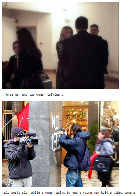
For instance, given the following image, the model should be able to produce acceptable captions describing the contents of the image. The captions should be good since various interpretations of the same image can exist.

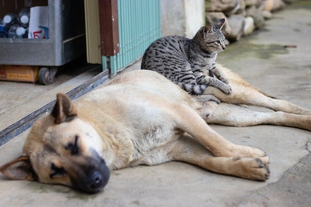
The captions for the above image can be:

• A cat and a dog are sleeping on the floor.
• A black cat is resting on a brown dog.
• A cat and a dog are resting at the garage entrance.

Approach to Creating the Model

The model is inspired by Implementing an image captioning model using a CNN and a Transformer and Image captioning with visual attention on TensorFlow. Some of the processes we will undertake:

• Source a dataset that has image, caption pairs.
• Visualize the dataset with Kangas to see its representation.
• Preprocess the images and captions.
• Resizing the images for pixel consistency through the model.
• Using a pre-trained CNN model to obtain image features.
• Create a Transformer encoder and decoder.
• Training the model.
• Generating captions using the trained model.
• Visualizing the model’s accuracy and loss.

The Dataset

There are several datasets available for image captioning tasks:

• Flickr8k: Has a little above 8k images paired with their respective captions.
• Flickr30k: Has over 30k images paired with their respective captions.
• MSCOCO: Have over 160k images paired with their respective captions.

These datasets have been widely used and are reliable in learning or building the image captioning model. We will stick with the Flickr8k dataset as it is more convenient for a broader range of audiences with inadequate resources for preparing and training more complicated datasets.

Download the dataset, and let’s get started!

%pip install opendatasets # to help download data directly from Kaggle

import opendatasets as od

# download
# Kaggle API key required
od.download("https://www.kaggle.com/datasets/adityajn105/flickr8k")

Visualizing the Dataset With Kangas

Kangas comes in handy for visualizing multimedia data. Unlike Pandas, Kangas comes packed with an effortless and straightforward way of visualizing image data (Kangas UI), and we do not have to rely on other libraries and packages to do so. I have provided the well-structured resources above to help you get started quickly.

First, install Kangas:

%pip install kangas

Next, import Kangas with an alias “kg“:

import kangas as kg

The base structure of Kangas is a DataGrid. However, we will first read the data as a Pandas DataFrame to process and add a column, after which we will read the DataFrame with Kangas to get the DataGrid.

Read the data. I am using Google Colab, hence the paths:

captions_file = '/content/flickr8k/captions.txt' 
df_captioned = pd.read_csv(captions_file)

# Add actual image path 
df_captioned['image'] = df_captioned['image'].apply(
lambda x: f'/content/flickr8k/Images/{x}')

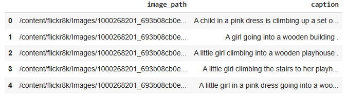
# Rename the 'image' column to 'image_path'
df_captioned.rename({'image':'image_path'}, axis=1, inplace=True)
df_captioned.head()

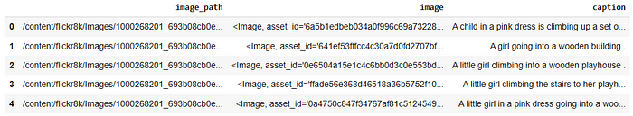
To visualize the images in Kangas, we need to convert the images to Kangas image assets with Image() or convert them to Pillow images(PIL).

# convert the images from the image paths
# to Kangas image assets
images= df_captioned['image_path'].map(
    lambda x: kg.Image(x)
)

# Add a new column with the image assets(actual images)
df_captioned.insert(loc=1, column='image', value=images)

df_captioned.head()

Let’s visualize some of the images with Kangas:

def viewRandomImages(samples=1):
  random_rows = df_captioned.sample(samples) #random images

  for idx, row in random_rows.iterrows():
    # view with Kangas
    image = kg.Image(row['image_path'])
    image.show()
    print('\n', row['caption'],'\n')

viewRandomImages(2) #view two images with captions

Kangas can read data in various formats into a DataGrid. Since we have the DataFrame, we will use Kangas’s read_dataframe() method to return a DataGrid. The best part of Kangas is the interactive Kangas UI. Instead of visualizing them individually, the UI creates a central place to view the images.

# view a shuffled DataGrid
dg_captioned = kg.read_dataframe(df_captioned.sample(frac=1))

# The dg.show() method to fire up the UI
dg_captioned.show()

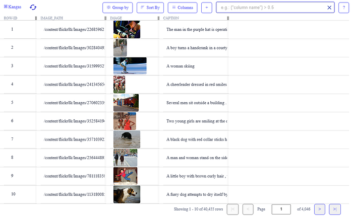
You can see that each image has a corresponding caption. On the UI, you can click on any image to view/zoom/apply grayscale, sort, or group the data as you wish to explore.

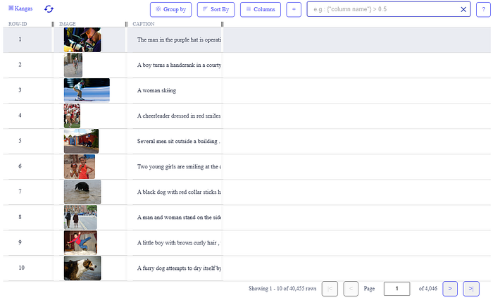
For instance, we can view the data without the “image_path” column. Just click on the “columns” tab and remove the row.

Perfect! Now that you have visualized how the data has been represented, it is time to create the model. But let’s first import all the libraries we will require.

import pandas as pd
import numpy as np
import matplotlib.pyplot as plt
import kangas as kg

import re
import tensorflow
import tensorflow as tf
from tensorflow import keras
from tensorflow.keras import layers
from tensorflow.keras.layers import TextVectorization

from tensorflow.keras.applications import efficientnet #Image feature extractor

Preparing the Dataset

The first step in building any model is converting the data into a carefully curated dataset to suit the model requirements before training. We require a paired dataset with images and their respective captions for an image captioning dataset.

Looking at the captions.txt file:

with open(captions_file) as caption_data:
  caption_data = caption_data.readlines()
  for data in caption_data[20:23]:
    print(data)

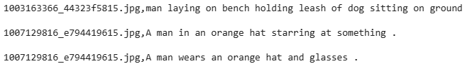
You notice that commas separate each image from its corresponding caption. Our goal is to separate the two entities.

Since we know that each image in the dataset has at least five captions to choose from, we will create a dictionary that maps each image (as keys) to its corresponding captions (as values). Also, for better consistency and model training, we will filter out the captions that are too short and those that are too long (marked as outliers) by predefining a sequence length.

If you are familiar with sequence-to-sequence tasks like machine translation, adding the start and end tokens to the captions will not surprise you. The start and end tokens act as explicit delimiters to the beginning and end of a sequence, thus helping the model identify the boundaries of the input sequence during training and inference.

def load_captions(caption_filename):

  with open(captions_file) as caption_data:
    caption_data = caption_data.readlines()

    mapping_dict = {} # dict to store image to caption mapping
    text_data = [] # stores a list of preocessed captions
    outlier_imgs = set()

    for line in caption_data:
      line = line.strip('\n').split(',') # split image and caption at the commas
      image_codeName, caption = line[0], line[1]
      image_name = os.path.join(image_paths, image_codeName)# create full path to image

      caption_tokens = caption.strip().split() # create tokens

      # filter the images using the caption lengths
      if len(caption_tokens) < 5 or len(caption_tokens) > sequenceLength:
        outlier_imgs.add(image_name)
        continue

      # get all .jpg images
      # add START and END tokens to each caption
      # convert the captions to lowercase
      if image_name.endswith('.jpg') and image_name not in outlier_imgs:
        caption = "<START> " + caption.strip().lower() + " <END>"
        text_data.append(caption)

        if image_name in mapping_dict:
            mapping_dict[image_name].append(caption)
        else:
            mapping_dict[image_name] = 

    for image_name in outlier_imgs:
      if image_name in mapping_dict:
        del mapping_dict[image_name]


    return mapping_dict, text_data

mapping_dict contains images (keys) mapped to their captions( values) while the text_data has all the preprocessed captions.

# mapped images to their caption
mapping_dict, text_data = load_captions(captions_file)

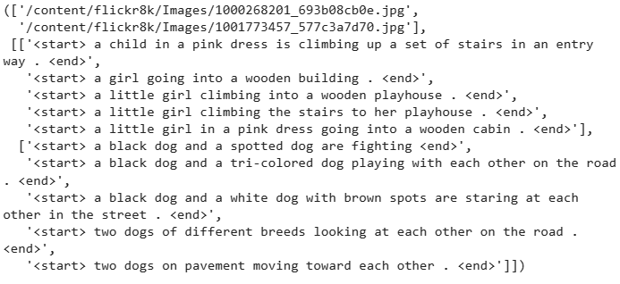
list(mapping_dict.keys())[:2], list(mapping_dict.values())[:2]

Let’s see the captions of one of the images:

mapping_dict['/content/flickr8k/Images/1000268201_693b08cb0e.jpg']

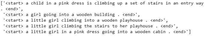
Each image is mapped to five corresponding captions.

Split the Data Into Training and Validation Sets

We will split the captioning data into two separate dictionaries for the training and validation data.

def train_val_split(caption_data, train_sample=0.8):

  images = list(caption_data.keys()) # gather all images

  train_sample = int(len(caption_data) * train_sample) # split

  training_set = {
      image_name: caption_data[image_name] for image_name in images[:train_sample]
  }
  validation_set = {
      image_name: caption_data[image_name] for image_name in images[train_sample:]
  }

  return training_set, validation_set

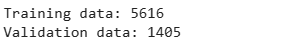
training_set, validation_set = train_val_split(mapping_dict)
print(f"Training data: {len(training_set)}\nValidation data: {len(validation_set)}")

Vectorizing the Data

To feed the data into the model, we need to vectorize it. That means that we need to convert the strings into integer sequences where each integer represents the index of a word in a vocabulary. TensorFlow provides the TextVectorization layer for this.

The layer learns the vocabulary from the captions through the adapt()method. The adapt() The method iterates over all captions, splits them into words, checks the frequency of each string value in the caption, and computes a vocabulary of their most frequently used words.

VOCAB_SIZE = 10000

def standardization(input):
    lowercase = tf.strings.lower(input)
    return tf.strings.regex_replace(lowercase, "[%s]" % re.escape(strip_chars), "")


strip_chars = "!\"#$%&'()*+,-./:;<=>?@[\]^_`{|}~"
strip_chars = strip_chars.replace("<", "")
strip_chars = strip_chars.replace(">", "")

vectorization = TextVectorization(
    max_tokens=VOCAB_SIZE,
    output_mode="int",
    output_sequence_length=sequenceLength,
    standardize=standardization,
)
vectorization.adapt(text_data)

We can check some vocabulary that has been computed after vectorization.

# Get some vocabulary
print(vectorization.get_vocabulary()[:15])

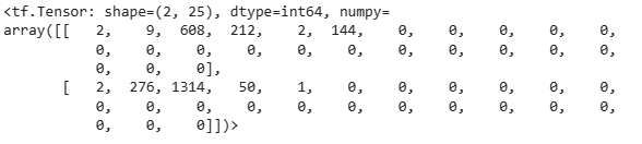
Let’s apply vectorization to some data to see the output sequences.

vectorizer = vectorization([['a dog sleeping under a tree'], ['a bird feeding small chicks']])
vectorizer

Create the tf.data.Dataset Pipeline

At this point, we need to transform, preprocess, and prepare the training and validation data for model training. We do this by creating a pipeline using the tf.data.Dataset API. With the pipeline, we can:

• Shuffle the dataset.
• Tokenize all captions for each image through the vectorization layer.
• Map the images to their respective captions.

In addition, we will create a function that will load each image and resize it to a fixed size for the model. That ensures that the same number of pixels represents all the images.

IMAGE_SIZE = (299, 299)
BATCH_SIZE = 64
EPOCHS = 30
AUTOTUNE = tf.data.AUTOTUNE

# load and resize each image to IMAGE_SIZE
def decode_and_resize(image_path):

  image = tf.io.read_file(image_path)
  image = tf.image.decode_jpeg(image, channels=3)
  image = tf.image.resize(image, IMAGE_SIZE)
  image = tf.image.convert_image_dtype(image, tf.float32)
  return image

# map each resized image to respective vectorized captions
def process_input(img_path, captions):
  return decode_and_resize(img_path), vectorization(captions)

# Function defining the transformation pipeline
def make_dataset(images, captions):
  dataset = tf.data.Dataset.from_tensor_slices((images, captions))
  dataset = dataset.shuffle(BATCH_SIZE * 8)
  dataset = dataset.map(process_input, num_parallel_calls=AUTOTUNE)
  dataset = dataset.batch(BATCH_SIZE).prefetch(AUTOTUNE)
  return dataset

# create transformed training and validation data
training_data = make_dataset(list(training_set.keys()), list(training_set.values()))

validation_data = make_dataset(list(validation_set.keys()), list(validation_set.values()))

Building the Model

The model will consist of three parts:

• An image feature extractor.
• The Transformer-based Encoder.
• The Transformer-based Decoder.

Image Feature Extractor

We will use an image model to extract features from each image. The model is pre-trained on ImageNet as an image classification model. However, in this case, we don’t need the classification layer but the last layer with feature maps. We will use the Keras EfficientNetB0 model.

Let’s take a look at the model results:

img_path = list(training_set.keys())[1]

model = efficientnet.EfficientNetB0(
      input_shape=(*IMAGE_SIZE, 3),
      include_top=False, weights = 'imagenet',
  )

test_img_batch = decode_and_resize(img_path)[tf.newaxis, :]
print(test_img_batch.shape)
print(model(test_img_batch).shape)

The feature extractor returns a feature map for each model.

Based on this model, we will create a new Convolutional Neural Network (CNN) Keras model for feature extraction. The CNN model will take as input the input tensor of feature maps from the EfficientNetB0 model.

def get_cnn_model():
  
  # include_top = False: return model without the 
  # classification layer
  model = efficientnet.EfficientNetB0(
      input_shape=(*IMAGE_SIZE, 3), include_top=False, weights = 'imagenet',

  )

  model.trainable = False
  model_out = model.output
  model_out = layers.Reshape((-1, model_out.shape[-1]))(model_out)
  cnn_model = keras.models.Model(model.input, model_out)
  return cnn_model

Next, we build a Transformer-based Encoder and Decoder.

Earlier sequence-to-sequence models implemented Recurrent Neural Networks (RNNs) like LSTM and GRU. The input sequence fed into those models was encoded into a fixed-length representation with information about the input sequence for output sequence generation. However, the fixed-length representations often posed limitations where the input sequence was too long and contained crucial information at different positions.

To fix that problem, an attention mechanism was added to enable the RNN models to focus on more relevant parts of the input sequence during the decoding process. So, instead of relying solely on the fixed-length representations, the attention mechanism calculates attention weights for each input position and computes a weighted sum of the input sequence’s encoder outputs. This weighted sum, often called the “attention context,” is an additional input to the decoder at each decoding step. However, the RNNs suffered from parallelism since they decoded one token at a time, making the model train slower, especially on long input sequences.

In this article, we implement the Transformer architecture for encoder and decoder. It is similar to the RNN model with attention, but the main difference is that Transformers entirely replace RNNs with an attention mechanism. That makes them parallelizable, and computations can happen simultaneously. Layer outputs can be computed in parallel instead of one at a time, like in RNNs.

To learn more about how Transformers work, you can read:

• “Attention is all you need” paper.
• Illustrated Transformer by Jay Alammar.

The Transformer-Based Encoder

We will pass the image features we have extracted as inputs to an encoder to generate new representations. The inputs first go through a self-attention layer. The layer creates three vectors (query, key, and value vectors), calculated by multiplying the embedding by the matrices from the training process. The self-attention layer adds MultiHeadAttention to enable the model to focus on different positions.

The self-attention layer can add variation in outputs. Adding layer normalization helps normalize the outputs to make them compatible with the original inputs (residue connection), which allows the preservation of important information and gradients.

class Encoder(keras.layers.Layer):
  def __init__(self, embedding_dim, dense_dim, num_heads):
    super().__init__()
    self.embedding_dim = embedding_dim
    self.dense_dim = dense_dim
    self.num_heads = num_heads

    # Create the attention layer
    self.attention = keras.layers.MultiHeadAttention(
        num_heads = num_heads, key_dim=embedding_dim, dropout=0.0
    )

    # Layer normalization
    self.layernorm1 = layers.LayerNormalization()
    self.layernorm2 = layers.LayerNormalization()

    self.dense = layers.Dense(embedding_dim, activation='relu')

    def call(self, inputs, training, mask=None):
      inputs = self.layernorm1(inputs)
      inputs = self.dense(inputs)

      attention_output = self.attention(
          query = inputs,
          value = inputs,
          keys = inputs,
          attention_mask = None,
          training = training
      )
      
      # residue connecttion
      # add actual inputs and self attention outputs
      # normalize them
      out = self.layernorm2(inputs + attention_output)
      return out

Positional Embedding Layer

Transformers do not have an inherent knowledge of order or position like RNNs. They would take the input sequence as Bag of Words, which may be indistinguishable. So before passing the image features as inputs to the encoder, we need to convert them into token embeddings and add positional information to each token. By doing so, the model can effectively encode both the content and the position of tokens in the input sequence, enabling it to capture positional relationships and dependencies in the data.

Below, we create two embedding layers for token embedding and one for positional embedding. The token embedding layer maps the tokens to dense vectors, while the positional embedding layer maps positions within the sequence of dense vectors.

class PositionalEmbedding(keras.layers.Layer):
  def __init__(self, seq_length, vocab_size, embedding_dim):
    super().__init__()
    self.token_embeddings = layers.Embedding(
        input_dim=vocab_size, output_dim=embedding_dim
    )
    self.position_embeddings = layers.Embedding(
        input_dim=seq_length, output_dim=embedding_dim
    )
    self.seq_length = seq_length
    self.vocab_size = vocab_size
    self.embedding_dim = embedding_dim
    self.embed_scale = tf.math.sqrt(tf.cast(embedding_dim, tf.float32))

  def call(self, inputs):
    length = tf.shape(inputs)[-1]
    positions = tf.range(start=0, limit=length, delta=1)
    embedded_tokens = self.token_embeddings(inputs)
    embedded_tokens = embedded_tokens * self.embed_scale
    embedded_positions = self.position_embeddings(positions)
    return embedded_tokens + embedded_positions

  def compute_mask(self, inputs, mask=None):
    return tf.math.not_equal(inputs, 0)

The Transformer-Based Decoder

The decoder is more complex to implement. It generates the output one by one while consulting the representation generated by the encoder. Like in an encoder, the decoder has a positional embedding layer and stack of layers.

The output of the top encoder is transformed into a set of attention vectors used in the “encoder-decoder attention” layer, enabling the decoder to focus on appropriate places in the input sequence. The decoder’s self-attention layer can only attend to earlier positions in the output sequence. That is done by masking future positions before the softmax step in the self-attention calculation.

class Decoder(keras.layers.Layer):
    @classmethod
      def add_method(cls, func):
        setattr(cls, func.__name__, func)
        return func

    def __init__(self, embedding_dim, ff_dim, num_heads):
        super().__init__()
        self.embedding_dim = embedding_dim
        self.ff_dim = ff_dim
        self.num_heads = num_heads
        self.attention1 = layers.MultiHeadAttention(
            num_heads=num_heads, key_dim=embedding_dim, dropout=0.1
        )
        self.attention2 = layers.MultiHeadAttention(
            num_heads=num_heads, key_dim=embedding_dim, dropout=0.1
        )
        self.ffn_layer1 = layers.Dense(ff_dim, activation="relu")
        self.ffn_layer2 = layers.Dense(embedding_dim)

        self.layernorm1 = layers.LayerNormalization()
        self.layernorm2 = layers.LayerNormalization()
        self.layernorm3 = layers.LayerNormalization()

        self.embedding = PositionalEmbedding(
              embedding_dim=512, seq_length=sequenceLength, vocab_size=VOCAB_SIZE
          )
        self.out = layers.Dense(VOCAB_SIZE, activation="softmax")

        self.dropout1 = layers.Dropout(0.3)
        self.dropout2 = layers.Dropout(0.5)
        self.supports_masking = True

      def call(self, inputs, encoder_outputs, training, mask=None):
        inputs = self.embedding(inputs)
        causal_mask = self.get_causal_attention_mask(inputs)

        if mask is not None:
            padding_mask = tf.cast(mask[:, :, tf.newaxis], dtype=tf.int32)
            combined_mask = tf.cast(mask[:, tf.newaxis, :], dtype=tf.int32)
            combined_mask = tf.minimum(combined_mask, causal_mask)

        attention_output1 = self.attention1(
            query=inputs,
            value=inputs,
            key=inputs,
            attention_mask=combined_mask,
            training=training,
        )
        out1 = self.layernorm1(inputs + attention_output1)

        attention_output2 = self.attention2(
            query=out1,
            value=encoder_outputs,
            key=encoder_outputs,
            attention_mask=padding_mask,
            training=training,
        )
        out2 = self.layernorm2(out1 + attention_output2)

        ffn_out = self.ffn_layer1(out2)
        ffn_out = self.dropout1(ffn_out, training=training)
        ffn_out = self.ffn_layer2(ffn_out)

        ffn_out = self.layernorm3(ffn_out + out2, training=training)
        ffn_out = self.dropout2(ffn_out, training=training)
        preds = self.out(ffn_out)
        return preds

Below, we write a method to generate a causal attention mask for the self-attention mechanism in a decoder layer. The causal attention mask ensures that each token can only attend to its previous positions and itself during self-attention, preventing information flow from future positions to past positions.

@Decoder.add_method
def get_causal_attention_mask(self, inputs):
        input_shape = tf.shape(inputs)
        batch_size, sequence_length = input_shape[0], input_shape[1]
        i = tf.range(sequence_length)[:, tf.newaxis] #(sequence_length, 1)
        j = tf.range(sequence_length) #(sequence_length,)

        #create the causal attention mask
        mask = tf.cast(i >= j, dtype="int32")
        mask = tf.reshape(mask, (1, input_shape[1], input_shape[1]))
        mult = tf.concat(
            [tf.expand_dims(batch_size, -1), tf.constant([1, 1], dtype=tf.int32)],
            axis=0,
        )
        return tf.tile(mask, mult)

The Model

In this section, we build the captioning model. The model combines the feature extractor from the CNN model (cnn_model method), the encoder, and the decoder to generate the captions for images. When we call the model for training, it should receive the image, caption pairs.

The model also calculates the loss and the average accuracy (by comparing the true labels and the predicted labels).

class ImageCaptioningModel(keras.Model):
  def __init__(
      self, cnn_model,
      encoder, decoder,
      num_captions_per_image=5
  ):

      super().__init__()
      self.cnn_model = cnn_model
      self.encoder = encoder
      self.decoder = decoder
      self.loss_tracker = keras.metrics.Mean(name="loss")
      self.acc_tracker = keras.metrics.Mean(name="accuracy")
      self.num_captions_per_image = num_captions_per_image
      self.image_aug = image_aug

  def calculate_loss(self, y_true, y_pred, mask):
    loss = self.loss(y_true, y_pred)
    mask = tf.cast(mask, dtype=loss.dtype)
    loss *= mask
    return tf.reduce_sum(loss) / tf.reduce_sum(mask)

  def calculate_accuracy(self, y_true, y_pred, mask):
    accuracy = tf.equal(y_true, tf.argmax(y_pred, axis=2))
    accuracy = tf.math.logical_and(mask, accuracy)
    accuracy = tf.cast(accuracy, dtype=tf.float32)
    mask = tf.cast(mask, dtype=tf.float32)
    return tf.reduce_sum(accuracy) / tf.reduce_sum(mask)

  def _compute_caption_loss_and_acc(self, img_embed, batch_seq, training=True):
    encoder_out = self.encoder(img_embed, training=training)
    batch_seq_inp = batch_seq[:, :-1]
    batch_seq_true = batch_seq[:, 1:]
    mask = tf.math.not_equal(batch_seq_true, 0)
    batch_seq_pred = self.decoder(
        batch_seq_inp, encoder_out, training=training, mask=mask
    )
    loss = self.calculate_loss(batch_seq_true, batch_seq_pred, mask)
    acc = self.calculate_accuracy(batch_seq_true, batch_seq_pred, mask)
    return loss, acc

  def train_step(self, batch_data):
    batch_img, batch_seq = batch_data
    batch_loss = 0
    batch_acc = 0

    if self.image_aug:
        batch_img = self.image_aug(batch_img)

    # 1. Get image embeddings
    img_embed = self.cnn_model(batch_img)

    # 2. Pass each of the five captions one by one to the decoder
    # along with the encoder outputs and compute the loss as well as accuracy
    # for each caption.
    for i in range(self.num_captions_per_image):
        with tf.GradientTape() as tape:
            loss, acc = self._compute_caption_loss_and_acc(
                img_embed, batch_seq[:, i, :], training=True
            )

            # 3. Update loss and accuracy
            batch_loss += loss
            batch_acc += acc

        # 4. Get the list of all the trainable weights
        train_vars = (
            self.encoder.trainable_variables + self.decoder.trainable_variables
        )

        # 5. Get the gradients
        grads = tape.gradient(loss, train_vars)

        # 6. Update the trainable weights
        self.optimizer.apply_gradients(zip(grads, train_vars))

    # 7. Update the trackers
    batch_acc /= float(self.num_captions_per_image)
    self.loss_tracker.update_state(batch_loss)
    self.acc_tracker.update_state(batch_acc)

    # 8. Return the loss and accuracy values
    return {"loss": self.loss_tracker.result(), "acc": self.acc_tracker.result()}

  def test_step(self, batch_data):
    batch_img, batch_seq = batch_data
    batch_loss = 0
    batch_acc = 0

    # 1. Get image embeddings
    img_embed = self.cnn_model(batch_img)

    # 2. Pass each of the five captions one by one to the decoder
    # along with the encoder outputs and compute the loss as well as accuracy
    # for each caption.
    for i in range(self.num_captions_per_image):
        loss, acc = self._compute_caption_loss_and_acc(
            img_embed, batch_seq[:, i, :], training=False
        )

        # 3. Update batch loss and batch accuracy
        batch_loss += loss
        batch_acc += acc

    batch_acc /= float(self.num_captions_per_image)

    # 4. Update the trackers
    self.loss_tracker.update_state(batch_loss)
    self.acc_tracker.update_state(batch_acc)

    # 5. Return the loss and accuracy values
    return {"loss": self.loss_tracker.result(), "acc": self.acc_tracker.result()}

  @property
  def metrics(self):
    # We need to list our metrics here so the `reset_states()` can be
    # called automatically.
    return [self.loss_tracker, self.acc_tracker]

cnn_model = get_cnn_model()
encoder = Encoder(embedding_dim=512, dense_dim=512, num_heads=1)
decoder = Decoder(embedding_dim=512, ff_dim=512, num_heads=2)
caption_model = ImageCaptioningModel(
    cnn_model=cnn_model, 
    encoder=encoder, 
    decoder=decoder
)

Train the Model

Since we have successfully implemented the model architecture, it is time to train it on the training data. We will monitor the model’s validation loss to gauge its performance. We do this by defining an EarlyStopping callback, which will stop the training if the model does not improve for three consecutive epochs (the model is overfitting).

# Define the loss function
cross_entropy = keras.losses.SparseCategoricalCrossentropy(
    from_logits=False, reduction="none"
)

# EarlyStopping criteria
early_stopping = keras.callbacks.EarlyStopping(
    patience=3, 
    restore_best_weights=True
    )

# Compile the model
caption_model.compile(
    optimizer=keras.optimizers.Adam(learning_rate=1e-4), 
    loss=cross_entropy)

# Fit the model
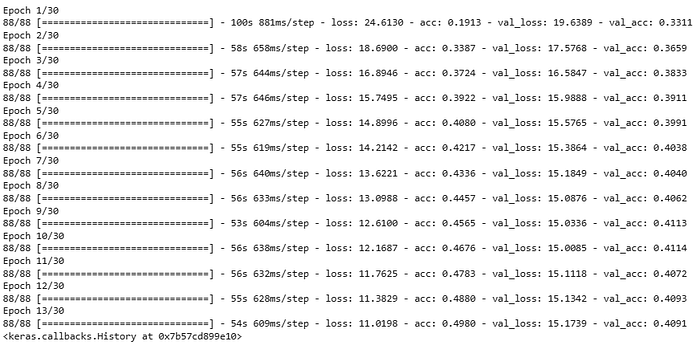
caption_model.fit(
    training_data,
    epochs=EPOCHS,
    validation_data=validation_data,
    callbacks=[early_stopping],
)

The accuracies and the losses at each training epoch.

Generating Captions

Finally, it’s time to predict captions for images using the trained Image captioning model. To caption an image with this model:

• Retrieve vocabulary from the training step and map each token position back to their corresponding words in the vocabulary.
• We will select a random image and its image features from the CNN model.
• Pass the image features to the encoder for encoding.
• Create a caption generation loop that generates tokens from <start> of the caption until the maximum decoded sentence length is reached or the end token <end> is generated.
  – Tokenize each caption with the vectorization layer.
  – Use the decoder to predict the next token in the sequence based on the encoded image features.

The model uses the Kangas Image() class to view each randomly selected image.

So, let’s add a “simple” method to do just that:

vocab = vectorization.get_vocabulary()
index_lookup = dict(zip(range(len(vocab)), vocab))
max_decoded_sentence_length = sequenceLength - 1
valid_images = list(validation_set.keys())


def generate_caption():
    # Select a random image from the validation dataset
    sample_img = np.random.choice(valid_images)

    # Read the image from the disk
    sample_img = decode_and_resize(sample_img)
    img = sample_img.numpy().clip(0, 255).astype(np.uint8)
    kg.Image(img).show()

    # Pass the image to the CNN
    img = tf.expand_dims(sample_img, 0)
    img = caption_model.cnn_model(img)

    # Pass the image features to the Transformer encoder
    encoded_img = caption_model.encoder(img, training=False)

    # Generate the caption using the Transformer decoder
    decoded_caption = "<start> "
    for i in range(max_decoded_sentence_length):
        tokenized_caption = vectorization([decoded_caption])[:, :-1]
        mask = tf.math.not_equal(tokenized_caption, 0)
        predictions = caption_model.decoder(
            tokenized_caption, encoded_img, training=False, mask=mask
        )
        sampled_token_index = np.argmax(predictions[0, i, :])
        sampled_token = index_lookup[sampled_token_index]
        if sampled_token == "<end>":
            break
        decoded_caption += " " + sampled_token

    decoded_caption = decoded_caption.replace("<start> ", "")
    decoded_caption = decoded_caption.replace(" <end>", "").strip().capitalize()
    print("PREDICTED CAPTION: ", decoded_caption)


# Check predictions for a few samples
generate_caption()
generate_caption()
generate_caption()

Predicted captions for each randomly selected image. We have displayed each image with Kangas.

Perfect!

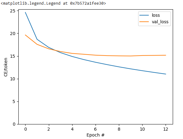
Visualize the Loss and Accuracy

plt.plot(caption_model.history.history['loss'], label='loss')
plt.plot(caption_model.history.history['val_loss'], label='val_loss')
plt.ylim([0, max(plt.ylim())])
plt.xlabel('Epochs')
plt.ylabel('CE/token')
plt.legend()

Loss:

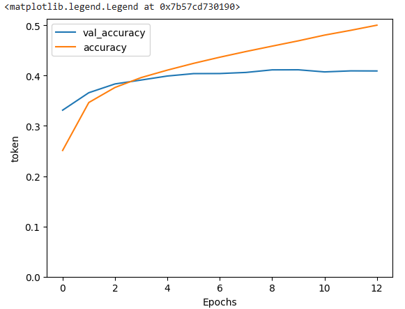
Accuracy:

plt.plot(caption_model.history.history['val_acc'], label='val_accuracy')
plt.plot(caption_model.history.history['acc'], label='accuracy')
plt.ylim([0, max(plt.ylim())])
plt.xlabel('Epochs')
plt.ylabel('CE/token')
plt.legend()

Final Thoughts

In this piece, we have learned to generate image captions with TensorFlow and Transformer based encoder and decoder. We have learned:

• How to visualize image data with Kangas and using the Kangas UI.
• How to preprocess image and caption data for proper model compatibility.
• How to create an image captioning model.