Customer Churn With Continuous Experiment Tracking

Introduction

In today’s competitive business environment, retaining customers is essential to a company’s success. Customer churn, or the rate at which customers leave your service, is an important metric that directly affects your business bottom line. To address this challenge, data scientists harness the power of machine learning to predict customer churn and develop strategies for customer retention.

In this article, we take a deep dive into a machine learning project aimed at predicting customer churn and explore how Comet ML, a powerful machine learning experiment tracking platform, plays a key role in increasing project success.

💡I write about Machine Learning on Medium || Github || Kaggle || Linkedin. 🔔 Follow “Nhi Yen” for future updates!

I. Customer Churn: Why Does It Matter?

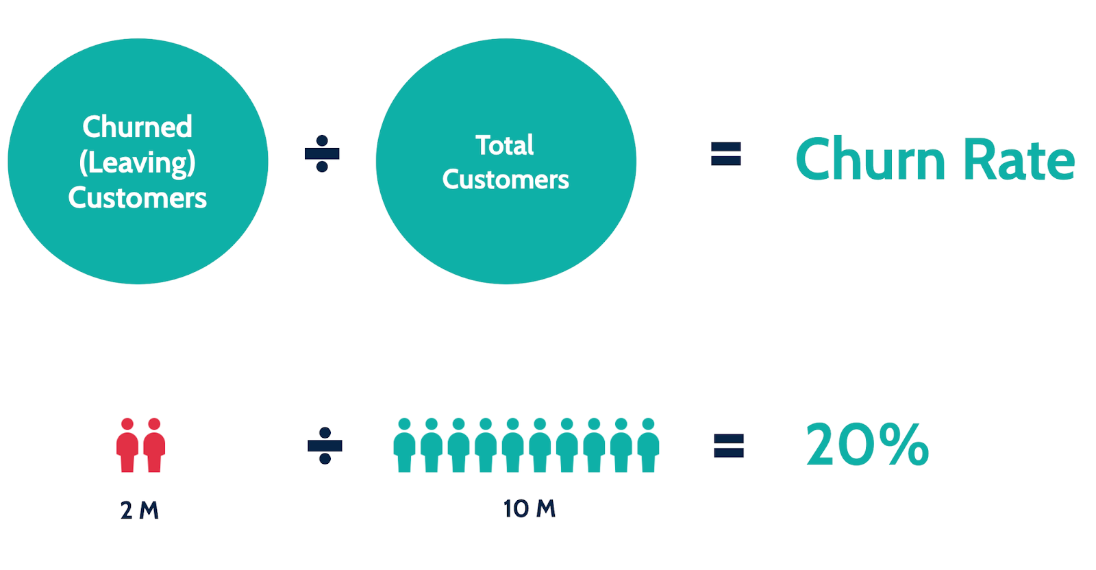
Customer churn refers to the phenomenon where customers stop using your service or product. This is an important metric for companies for the following reasons:

• Impact on revenue: Loss of customers reduces revenue and growth opportunities.
• Acquisition costs: Acquiring new customers is usually more expensive than retaining existing customers.
• Customer Feedback: Understanding why customers leave provides valuable information to improve your service.

II. Customer Churn Project and Dataset

1. Project Objective

The goal of our project is to predict customer churn for telecommunications companies using a model stacking approach. Model stacking involves training multiple machine learning models and using another model to combine their predictions to improve accuracy.

2. Dataset

This project uses the “Telco Customer Churn” dataset available on Kaggle. This dataset contains information about telecom customers, such as contract type, monthly fee, and whether the customer has canceled.

Tired of manually tracking your prompts and prompt variables? Try CometLLM, a free, open-source tool to log, visualize, and search your LLM prompts and metadata.

III. Continuous Experiment Tracking for Customer Churn with Comet ML

Comet ML is a versatile tool that helps data scientists optimize machine learning experiments. In our project, we use Comet ML to:

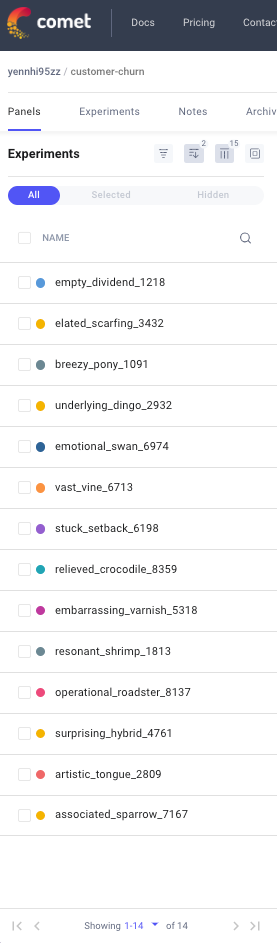
1. Experiment Tracking

Comet ML has a section where you can create and manage experiments. This is where you record information about your experiment, such as metrics, hyperparameters, and other relevant details.

Comet ML allows you to record several metrics such as precision, log loss, and ROC AUC score at each step of your experiment. This detailed log is invaluable for tracking model performance and understanding how changes impact results.

2. Visualization

Within Comet ML, you need tools to visualize the results of your experiments, such as tables and graphs showing metrics over time or across different runs.

3. Hyperparameter Tuning

Hyperparameter optimization is critical to model performance. Comet ML seamlessly integrates with Optuna, an automated hyperparameter optimization framework. This allows you to efficiently tune the hyperparameters of your machine learning model.

👉 Read more about CometML — HERE

You might be interested in:

• Logging — The Effective Management of Machine Learning Systems
• Hyperparameter Tuning in Machine Learning: A Key to Optimize Model Performance

IV. Step-by-step guide: How the customer churn project works.

👉 The entire code can be found on both GitHub and Kaggle.

Here’s an overview of the steps we follow in our project:

1. Import Libraries

First, import the required Python libraries, such as Comet ML, Optuna, and scikit-learn. These libraries provide tools for data pre-processing, model training, and hyperparameter tuning.

!pip install -q optuna comet_ml
import optuna
import comet_ml
from comet_ml import Experiment

import pandas as pd
import numpy as np
import matplotlib.pyplot as plt
import seaborn as sns
from sklearn.model_selection import train_test_split
from sklearn.preprocessing import StandardScaler, OneHotEncoder
from sklearn.linear_model import LogisticRegression
from sklearn.ensemble import RandomForestClassifier, GradientBoostingClassifier
from sklearn.svm import SVC
from sklearn.metrics import accuracy_score, log_loss, roc_auc_score
from sklearn.model_selection import GridSearchCV
from sklearn.ensemble import StackingClassifier
from sklearn.metrics import accuracy_score, log_loss

from kaggle_secrets import UserSecretsClient

# Set display options to show all columns
pd.set_option('display.max_columns', None)

user_secrets = UserSecretsClient()
comet_api_key = user_secrets.get_secret("Comet API Key")

experiment = Experiment(
    api_key= YOUR_COMET_API,
    project_name= YOUR_PROJECT_NAME,
    workspace= YOUR_WORKSPACE
)

In this project, I use a Kaggle notebook to schedule daily runs, and Comet ML records each run as an experiment. In a typical MLOps project, similar scheduling is essential to handle new data and track model performance continuously.

2. Load and Explore Data

We load the Telco Customer Churn dataset and perform exploratory data analysis (EDA). EDA is essential for gaining insights into the dataset’s characteristics and identifying any data preprocessing requirements.

During this step, for each plot, I use experiment.log_figure(figure=plt) to log the plot to Comet. You can access these plots by going to [Experiment] > Graphics.

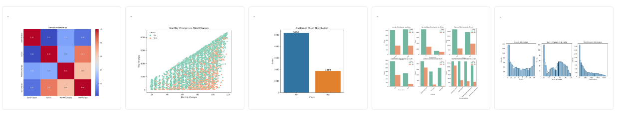
For the final experiment I have run, this is the results:

#1. Customer Churn Distribution

This plot shows the distribution of churn vs. non-churn customers. In it, you can see the number of customers who have churned (left the telecom service) and those who have not.

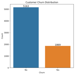
The dataset shows an imbalance with 5,174 non-churned and 1,869 churned customers. Imbalanced data may require special model training techniques, like oversampling or undersampling, to handle class imbalance effectively.

#2. Numeric Feature Distribution

These histograms show the distribution of numeric features (tenure, MonthlyCharges, and TotalCharges) for the entire dataset.

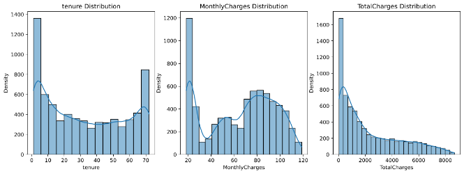
You can observe how these numeric features are distributed. For instance, understanding the distribution of MonthlyCharges and TotalCharges can help in pricing strategy decisions. Are there clusters of customers with different spending patterns?

#3. Categorical Feature Distribution

These plots show the distribution of categorical features (gender, SeniorCitizen, Partner, Dependents, Contract, PaymentMethod) split by churn status.

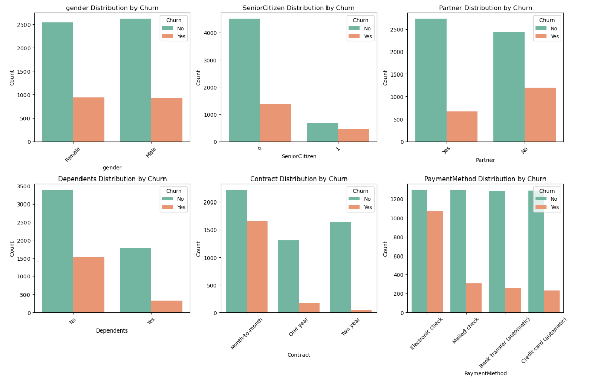
These plots provide insights into how different categories of customers (e.g., seniors vs. non-seniors, customers with partners vs. without) are distributed in terms of churn. You can identify potential customer segments that are more likely to churn.

#4. Correlation Heatmap:

The heatmap displays the correlation between numeric features in the dataset.

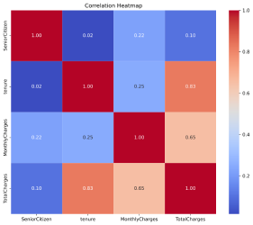
Understanding feature correlations can help in feature selection. For instance, if monthly charges and total charges are highly correlated, you might choose to keep only one of them to avoid multicollinearity in your models. It also helps identify which features might be more important in predicting churn.

#5. Monthly Charges vs. Total Charges:

This scatterplot shows the relationship between monthly charges and total charges, with points colored by churn status.

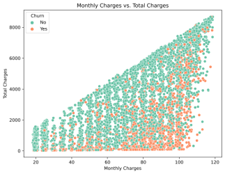
In the graph above, it appears that customers who have higher Total Charges are less likely to churn. This suggests that long-term customers who spend more are more loyal. You can use this insight to focus on retaining high-value, long-term customers by offering loyalty programs or incentives.

These business insights derived from EDA can guide feature engineering and model selection for your churn prediction project. They help you understand the data’s characteristics and make informed decisions to optimize customer retention strategies.

3. Preprocessing

Data preprocessing is a critical step. In it, we encode categorical features, scale numerical features, and split the data into training and validation sets.

# Encode categorical features, scale numerical features

encoder = OneHotEncoder(handle_unknown="ignore", sparse=False)
scaler = StandardScaler()

X_train, X_val, y_train, y_val = train_test_split(data.drop("Churn", axis=1), data["Churn"], test_size=0.2, random_state=42)

X_train_encoded = encoder.fit_transform(X_train[categorical_features])
X_val_encoded = encoder.transform(X_val[categorical_features])

X_train_scaled = scaler.fit_transform(X_train[numerical_features])
X_val_scaled = scaler.transform(X_val[numerical_features])

X_train_processed = np.concatenate((X_train_encoded, X_train_scaled), axis=1)
X_val_processed = np.concatenate((X_val_encoded, X_val_scaled), axis=1)

4. Model Training

We train multiple machine learning models, including Logistic Regression, Random Forest, Gradient Boosting, and Support Vector Machine. These models serve as the basis for our ensemble approach.

Logistic Regression (logreg):

• Simple and interpretable model.
• Well-suited for binary classification tasks like churn prediction.
• Helps understand how features impact the chance of churn.

Random Forest Classifier (rf):

• Ensemble method combining multiple decision trees.
• Handles mixed feature types (categorical and numerical).
• Resistant to overfitting, good for complex datasets.

Gradient Boosting Classifier (gb):

• Sequential ensemble building strong predictive power.
• Captures complex relationships in data.
• Works well for various types of datasets.

Support Vector Machine (svm):

• Versatile model for linear and non-linear data.
• Can find complex decision boundaries.
• Useful when patterns between churn and non-churn are intricate.

Modeling Stacking

In the project, I am stacking models such as random forests, gradient boosting, and support vector machines, which each have different characteristics and can capture different aspects of the customer churn problem. This approach can help you achieve a more accurate and robust churn prediction model, ultimately leading to better customer retention strategies and business outcomes.

Comet ML comes into play by allowing you to log the models’ performance, hyperparameters, and other metadata.

5. Hyperparameter Tuning & Ensemble Modeling

Using Optuna, we optimize hyperparameters for the individual models. This step ensures that our models are fine-tuned for maximum accuracy.

We create a stacking ensemble of models to combine their predictions. This will enhance our predictive performance.

def objective(trial):
    # Define hyperparameter search space for individual models
    rf_params = {
        'n_estimators': trial.suggest_int('rf_n_estimators', 100, 300),
        'max_depth': trial.suggest_categorical('rf_max_depth', [None, 10, 20]),
        'min_samples_split': trial.suggest_int('rf_min_samples_split', 2, 10),
        'min_samples_leaf': trial.suggest_int('rf_min_samples_leaf', 1, 4),
    }

    gb_params = {
        'n_estimators': trial.suggest_int('gb_n_estimators', 100, 300),
        'learning_rate': trial.suggest_float('gb_learning_rate', 0.01, 0.2),
        'max_depth': trial.suggest_categorical('gb_max_depth', [3, 4, 5]),
    }

    svm_params = {
        'C': trial.suggest_categorical('svm_C', [0.1, 1, 10]),
        'kernel': trial.suggest_categorical('svm_kernel', ['linear', 'rbf']),
    }

    # Create models with suggested hyperparameters
    rf = RandomForestClassifier(**rf_params)
    gb = GradientBoostingClassifier(**gb_params)
    svm = SVC(probability=True, **svm_params)

    # Train individual models
    rf.fit(X_train_processed, y_train)
    gb.fit(X_train_processed, y_train)
    svm.fit(X_train_processed, y_train)

    # Evaluate individual models on validation data
    rf_predictions = rf.predict(X_val_processed)
    gb_predictions = gb.predict(X_val_processed)
    svm_predictions = svm.predict(X_val_processed)

    # Calculate accuracy and ROC AUC for individual models
    rf_accuracy = accuracy_score(y_val, rf_predictions)
    gb_accuracy = accuracy_score(y_val, gb_predictions)
    svm_accuracy = accuracy_score(y_val, svm_predictions)

    rf_roc_auc = roc_auc_score(y_val, rf.predict_proba(X_val_processed)[:, 1])
    gb_roc_auc = roc_auc_score(y_val, gb.predict_proba(X_val_processed)[:, 1])
    svm_roc_auc = roc_auc_score(y_val, svm.predict_proba(X_val_processed)[:, 1])

    # Create a stacking ensemble with trained models
    estimators = [
        ('random_forest', rf),
        ('gradient_boosting', gb),
        ('svm', svm)
    ]

    stacking_classifier = StackingClassifier(estimators=estimators, final_estimator=LogisticRegression())

    # Train the stacking ensemble
    stacking_classifier.fit(X_train_processed, y_train)

    # Evaluate the stacking ensemble on validation data
    stacking_predictions = stacking_classifier.predict(X_val_processed)
    stacking_accuracy = accuracy_score(y_val, stacking_predictions)
    stacking_roc_auc = roc_auc_score(y_val, stacking_classifier.predict_proba(X_val_processed)[:, 1])

    # Log parameters and metrics to Comet ML
    experiment.log_parameters({
        'rf_n_estimators': rf_params['n_estimators'],
        'rf_max_depth': rf_params['max_depth'],
        'rf_min_samples_split': rf_params['min_samples_split'],
        'rf_min_samples_leaf': rf_params['min_samples_leaf'],
        'gb_n_estimators': gb_params['n_estimators'],
        'gb_learning_rate': gb_params['learning_rate'],
        'gb_max_depth': gb_params['max_depth'],
        'svm_C': svm_params['C'],
        'svm_kernel': svm_params['kernel']
    })

    experiment.log_metrics({
        'rf_accuracy': rf_accuracy,
        'gb_accuracy': gb_accuracy,
        'svm_accuracy': svm_accuracy,
        'rf_roc_auc': rf_roc_auc,
        'gb_roc_auc': gb_roc_auc,
        'svm_roc_auc': svm_roc_auc,
        'stacking_accuracy': stacking_accuracy,
        'stacking_roc_auc': stacking_roc_auc
    })

    # Return the negative accuracy as Optuna aims to minimize the objective
    return -stacking_accuracy

As you can see, Comet ML can help you log and track the hyperparameter tuning process, allowing you to compare different runs and select the best hyperparameters.

6. Optimization Results

Next, we display the best hyperparameters and accuracy scores achieved through hyperparameter tuning, providing transparency in our model selection process.

from tabulate import tabulate

# Create and optimize the study
study = optuna.create_study(direction='minimize')  # Adjust direction based on your optimization goal
study.optimize(objective, n_trials=100)  # You can adjust the number of trials

# Get the best hyperparameters and results
best_rf_params = study.best_params
best_accuracy = -study.best_value  # Convert back to positive accuracy

# Convert the dictionary to a list of key-value pairs for tabulation
param_table = [(key, value) for key, value in best_rf_params.items()]

# Display the best_rf_params table
best_rf_params = tabulate(param_table, headers=["Parameter", "Value"], tablefmt="grid")

print(f"Best RF Hyperparameters:\n{best_rf_params}")
print(f"Best Accuracy: {best_accuracy}")

7. End Experiment

Finally, we conclude the Comet ML experiment, ensuring all relevant information is logged for future reference.

experiment.end()

8. Business Insights

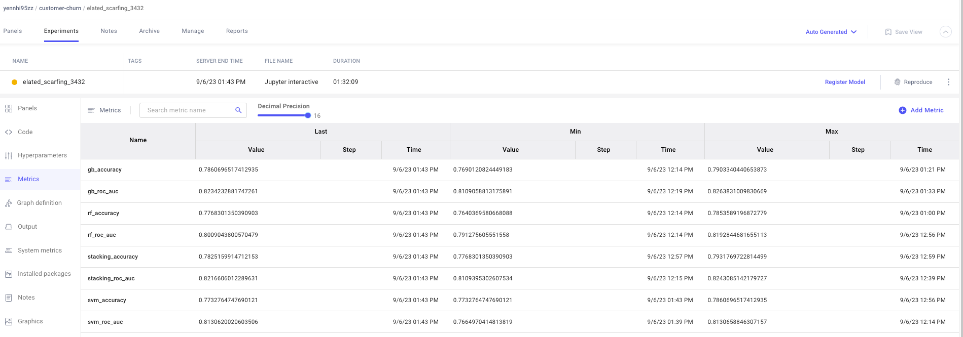
After running an experiment, you can check the results by going to the Respective Experiment > Experiment > Dashboards or theRespective Experiment > Experiment > Metrics.

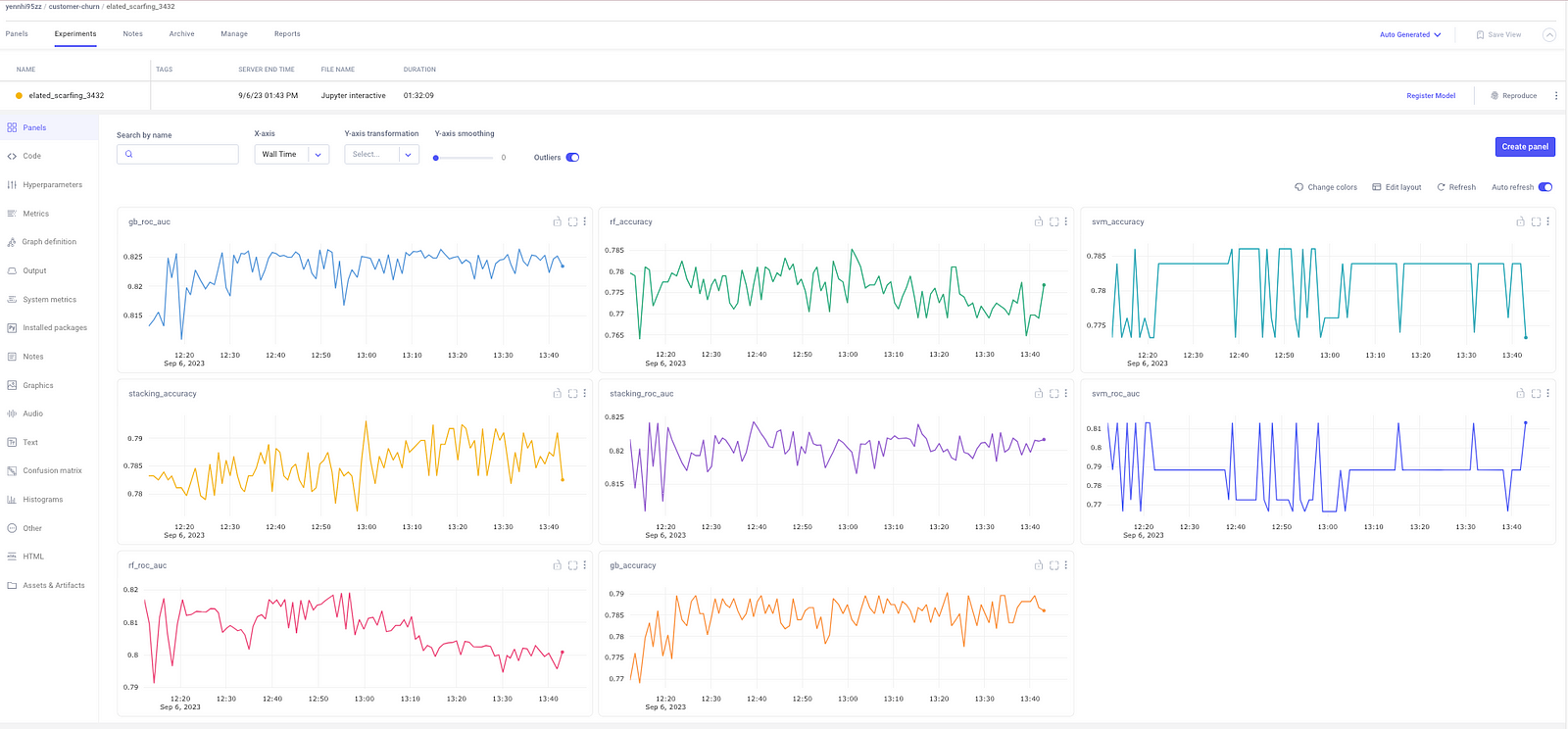
Now, lets explore the business insights based on these optimization results:

#1. Model Selection:

• The project aimed to predict customer churn, a critical concern for telecom companies. Model stacking was used to enhance prediction accuracy.
• From the optimization results, we can see that Gradient Boosting (gb) achieved the highest accuracy (0.786) and ROC AUC (0.823) scores among individual models. It’s a promising choice for predicting customer churn due to its good performance.

#2. Ensemble Modeling:

• Stacking models (stacking_accuracy) achieved an accuracy of 0.783, slightly higher than the individual Random Forest (0.777) and Support Vector Machine (0.773) models.
• The stacking ensemble also outperformed in terms of ROC AUC (0.822), indicating its ability to balance false positives and true positives, which is crucial for customer churn prediction.

#3. Hyperparameter Tuning:

• Hyperparameter tuning was conducted to optimize model performance.
• The optimized models, particularly Gradient Boosting and Random Forest, show improved accuracy compared to their default configurations.

# 4. Decision-Making Insights:

• Telecom companies can use these models to identify customers at risk of churn.
• Strategies can be developed to retain high-risk customers, such as offering tailored promotions or better customer service.
• Insights from Gradient Boosting, which performed the best, can help identify key factors influencing churn, allowing the company to take proactive measures.
• The stacking ensemble provides robust predictions, combining the strengths of multiple models.

#5. Monitoring and Continuous Improvement:

• Regular monitoring of churn prediction using these models can help the telecom company adapt to changing customer behaviors.
• Continuous hyperparameter tuning and model retraining can further enhance predictive accuracy over time.

Conclusion

In this article, we explored a churn prediction project using machine learning and Comet ML. A combination of model stacking, hyperparameter tuning, and insightful EDA will enable you to build robust churn prediction models.

Predicting customer churn is just one application of machine learning in business, but the impact is significant. By leveraging tools like Comet ML, data scientists can optimize models and gain insights that ultimately contribute to improved customer retention strategies and business results.

If you want to learn more about the world of machine learning and data science, keep an eye out for future articles. Remember that the power of data is in your hands and with the right tools and techniques you can make data-driven decisions that drive business success.