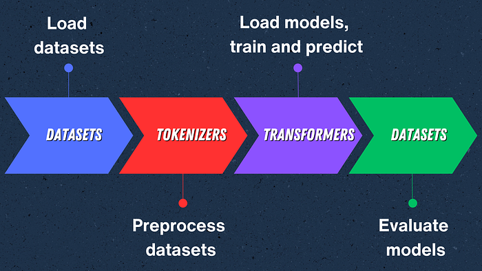
LLMs such as GPT, BERT, and Llama 2 are a game changer in AI. You can build AI tools like ChatGPT and Bard using these models. But you need to fine-tune these language models when performing your deep learning projects. This is where AI platforms come in.

Today, I’ll show you how to build an end-to-end text classification project. Here are the topics we’ll cover in this article:

• Fine-tuning the BERT model with the Transformers library for text classification.
• Building a web app with the Gradio.
• Monitoring this app with Comet.

After creating the app, it will look like the one below:

You can leverage this Kaggle notebook to follow the code with me and look at this repo to review the project files.

Let’s start by installing the necessary platforms.

Step 1. Installing Required Libraries

The first thing we’re going to do is install the necessary libraries. This is very easy to do with the pip package manager, as shown below:

!pip install -q comet_ml transformers datasets gradio

After that, let’s go ahead and initialize the platforms we will use.

Step 2. Initialize Comet and Hugging Face

To track our hyperparameters and monitor our app, we’ll use Comet. To do this, we first need to initialize it, as shown below:

import comet_ml

# Initializing the project
comet_ml.login(project_name="text-classification-with-transformers")

After running this snippet, you need to enter your Comet API key. Go to Comet and create a free account to get your API key.

Plus, after training our LLM model, we’ll push it to Hugging Face Spaces, which allows you to host your ML demo apps on your profile.

Logging in to Hugging Face with the notebook_login method is very easy. To do this, use your Hugging Face API key. If you don’t have your API key, you can get it for free here.

from huggingface_hub import notebook_login

# Logining Hugging Face
notebook_login()

Nice, we’ve initialized the platform we’ll use. Let’s move on to loading the dataset.

Step 3. Load Data

The dataset we will use is a movie review dataset called rotten tomatoes. Fortunately, this dataset is available in the datasets library. All we need to do is load this dataset with the load_dataset method. Let’s do this:

from datasets import load_dataset

# Loading the dataset
raw_datasets = load_dataset("rotten_tomatoes")

Great, our data is loaded. Let’s take a look at this data:

raw_datasets

# Output:
""""
DatasetDict({
    train: Dataset({
        features: ['text', 'label'],
        num_rows: 8530
    })
    validation: Dataset({
        features: ['text', 'label'],
        num_rows: 1066
    })
    test: Dataset({
        features: ['text', 'label'],
        num_rows: 1066
    })
})
"""

As you can see, data is very similar to a Python dictionary, where each key corresponds to a different dataset. We can utilize the usual dictionary syntax to look at a single split:

# Looking at the first sample of the training set
raw_datasets["train"][0]

# Output:
"""
{'text': 'the rock is destined to be the 21st century\'s new " conan " and that he\'s going to make a splash even greater than arnold schwarzenegger , jean-claud van damme or steven segal .',
 'label': 1}
"""

Awesome, we’ve seen the first sample of the training dataset. Now, to gain more insight about the data, let’s convert it to Pandas DataFrame

Step 4. Understand Data

Understanding data is one of the most important stages of the data analysis lifecycle. To do this, there is no doubt that Pandas are king.

From Datasets to Pandas DataFrames

First, let me convert the data into Pandas DataFrame with the set_formatmethod as follows:

import pandas as pd

# Converting the dataset into Pandas dataframe
raw_datasets.set_format(type="pandas")
df = raw_datasets["train"][:]
df.head()

As you can see, the data contains only two columns: text and label. Let’s move on to exploring the class distribution.

Looking at the Label Distribution

The simplest way to understand data is to visualize it. Let’s draw a bar chart with Matplotlib to look at the label distribution.

import matplotlib.pyplot as plt

# Visualizing the frequency of classes
df["label_name"].value_counts(ascending=True).plot.barh()
plt.title("Frequency of Classes")
plt.show()

As you can see, the distribution of labels is balanced.

How Long Are Our Texts?

The model we’ll use is DistilBERT. Like other transformer models, this model has a maximum input text length. This number is 512.

Let’s take a look at the distribution of words per review:

# Visualizing words per review
df["Words Per Review"] = df["text"].str.split().apply(len)
df.boxplot("Words Per Review", by="label_name", grid=False, showfliers=False,
           color="black")
plt.suptitle("")
plt.xlabel("")
plt.show()

As you can see, most reviews are around 15 words long, and the longest reviews are well below DistilBERT’s maximum sequence size.

Nice, we examined our data. Since we no longer need the DataFrame format, let’s reset the format of our dataset:

# Reseting the dataset format
raw_datasets.reset_format()

Now, we’re ready to preprocess data. Let’s do this.

Step 5. Data Preprocessing

Deep learning models don’t like raw strings as input. Instead, they want the text to be encoded as numerical representations. This is where tokenization comes in. Tokenization is a way of breaking sentences into smaller units called tokens.

We are lucky that Transformers contains an AutoTokenizer class. This class helps you quickly load the tokenizer associated with a pre-trained model. All you need to do is call your model’s from_pretrained method. In our case, let’s start by loading the tokenizer for DistilBERT as follows:

from transformers import AutoTokenizer

# Loading the DistilBERT tokenizer 
checkpoint = "distilbert-base-uncased"
tokenizer = AutoTokenizer.from_pretrained(checkpoint)

Okay, our tokenizer is ready to apply the whole corpus. Let’s create a preprocessing function and pass the truncation parameter to it. This parameter will truncate the texts to the model’s maximum input size.

After creating the function, let’s tokenize our datasets using the map method with the batched parameter. This parameter speeds up the function by simultaneously processing multiple dataset elements.

# Creating a function for tokenization
def tokenize_function(examples):
    return tokenizer(examples["text"], truncation=True)

# Applying the function to the entire dataset
tokenized_datasets = raw_datasets.map(tokenize_function, batched=True)

Nice, we tokenized our datasets. It’s time to create a batch of examples with DataCollatorWithPadding.This method will dynamically pad the sentences received instead of padding the entire dataset to the maximum length.

from transformers import DataCollatorWithPadding

# Padding
data_collator = DataCollatorWithPadding(tokenizer=tokenizer)

Awesome, we preprocessed the datasets. Let’s go ahead and create the evaluation function.

Step 6. Evaluation Function

As you know, metrics help us evaluate the performance of the model. For this analysis, we’ll compute the accuracy, precision, recall, and f1 metrics.

Let’s create a function named compute_metrics to track metrics during training. To do this, we will leverage the Scikit-Learn and Comet libraries.

from sklearn.metrics import accuracy_score, precision_recall_fscore_support

# Indexing to example function
def get_example(index):
    return tokenized_datasets["test"][index]["text"]

# Creating a function to compute metrics
def compute_metrics(pred):
    experiment = comet_ml.get_global_experiment()

    labels = pred.label_ids
    preds = pred.predictions.argmax(-1)
    precision, recall, f1, _ = precision_recall_fscore_support(
        labels, preds, average="macro"
    )
    acc = accuracy_score(labels, preds)

    if experiment:
        epoch = int(experiment.curr_epoch) if experiment.curr_epoch is not None else 0
        experiment.set_epoch(epoch)
        experiment.log_confusion_matrix(
            y_true=labels,
            y_predicted=preds,
            file_name=f"confusion-matrix-epoch-{epoch}.json",
            labels=["negative", "positive"],
            index_to_example_function=get_example,
        )

    return {"accuracy": acc, "f1": f1, "precision": precision, "recall": recall}

Great, we defined the performance metrics. We’ll use this function in the model training step. Let’s move on to building the model.

Step 7. Transformer Model

Trust me, it’s straightforward to fit a model using Transformers.

First, instantiate your model using the AutoModelForSequenceClassificationclass and then fine-tune this model according to your data with the num_labels parameter. That’s simple, right?

In our case, we’ll pass two to this parameter because the labels of our dataset are two classes. Also, let’s use id2label and label2id to match the expected IDs to their labels.

from transformers import AutoModelForSequenceClassification

# Mapping ids to labels 
id2label = {0: "NEGATIVE", 1: "POSITIVE"}
label2id = {"NEGATIVE": 0, "POSITIVE": 1}

# Building the model
model = AutoModelForSequenceClassification.from_pretrained(
              checkpoint, num_labels=2, id2label=id2label, label2id=label2id)

Cool, we loaded our pre-trained model. Let’s go ahead and start training this model.

Step 8. Run Training

It’s time to train the model. First, let’s define the training parameters using the TrainingArguments class. In this step, we will set push_to_hub=True to push this model to our Hugging Face Hub and report_to=["comet_ml"]to monitor our hyperparameters in the Comet Dashboard.

After that, what we’re going to do is instantiate our model and fine-tune it with the Trainer.

Lastly, we’re going to call the train method to start training. That’s it.

from transformers import TrainingArguments, Trainer

# Setting Comet enviroment variables
%env COMET_MODE=ONLINE
%env COMET_LOG_ASSETS=TRUE

# Setting training arguments
training_args = TrainingArguments(
    output_dir="my_distilbert_model",
    learning_rate=2e-5,
    per_device_train_batch_size=16,
    per_device_eval_batch_size=16,
    num_train_epochs=3,
    weight_decay=0.01,
    evaluation_strategy="epoch",
    save_strategy="epoch",
    load_best_model_at_end=True,
    push_to_hub=True,
    report_to=["comet_ml"],
)

# Creating a trainer object
trainer = Trainer(
    model=model,
    args=training_args,
    train_dataset=tokenized_datasets["train"],
    eval_dataset=tokenized_datasets["test"],
    compute_metrics=compute_metrics,
    data_collator=data_collator,
)

# Training the model
trainer.train()

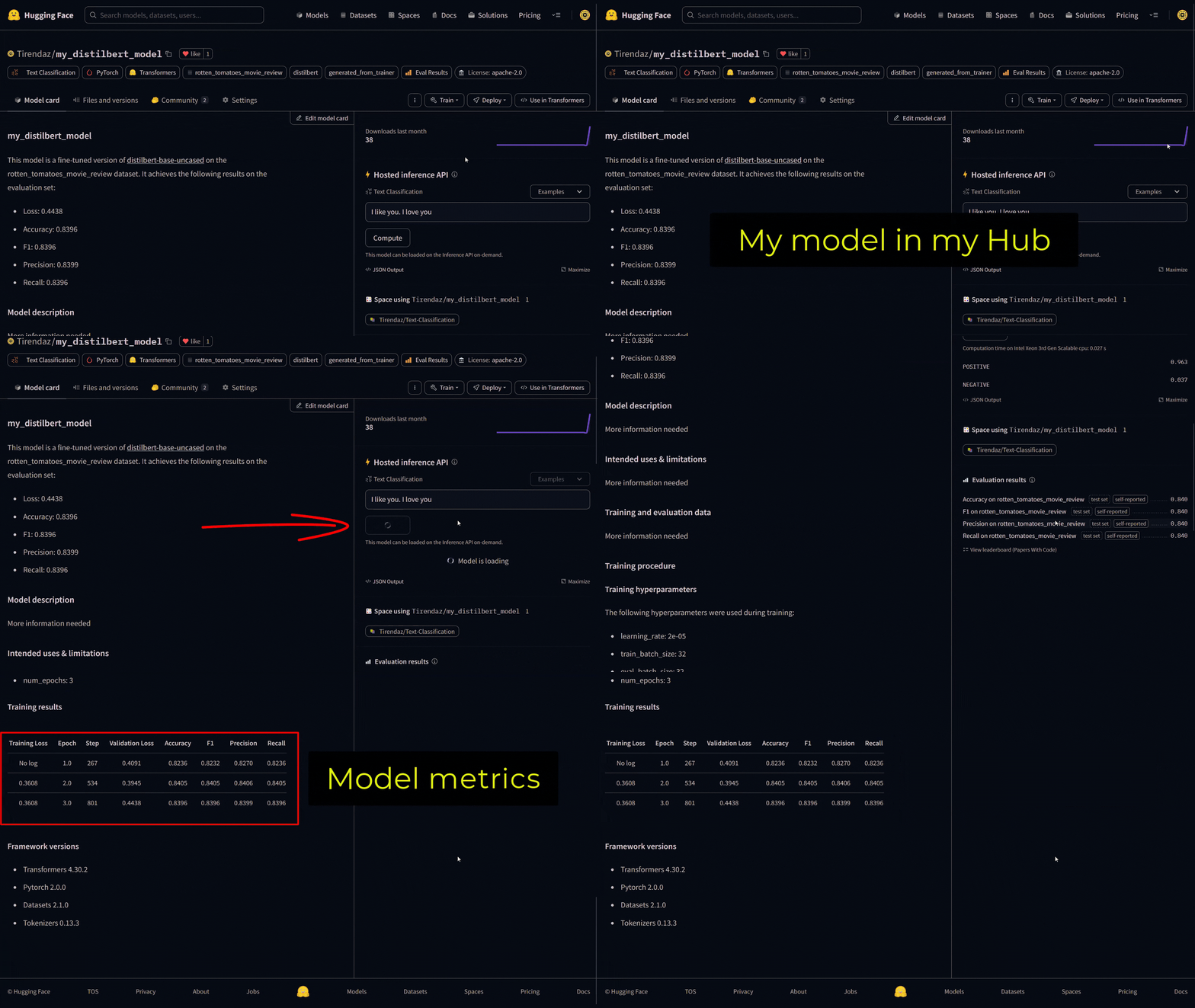
Voilà, our model was trained, and metrics were calculated for each epoch. As you can see, the performance of our model is not bad.

It’s time to push our model to the HUB to share with everyone, as shown below:

# Pushing the model
trainer.push_to_hub()

Our model looks like this in my Hub:

Let’s take a look at how to predict the label of a text that the model has not seen before.

Step 9. Inference

We now have a model on the Hugging Face Hub. It’s time to make a prediction using this model. The easiest way to do this is to use a pipeline. All we have to do is pass our model to it. Let’s do this:

from transformers import pipeline

# Creating a text
text = "This is a great movie. It may be my favourite."

# Predicting the label
classifier = pipeline("sentiment-analysis", 
                       model="Tirendaz/my_distilbert_model")
classifier(text)

# Output:
# [{'label': 'POSITIVE', 'score': 0.971620500087738}]

As you can see, the prediction was made, and the score for this prediction was calculated. Our model correctly predicted the label of the text.

Let’s move on to deploying our model with Gradio.

Step 10. Deploy

In the final step, we’ll walk you through how to share our model with the community. Gradio is king when it comes to sharing machine learning models.

It’s important to note that you can display your app on Hugging Face Hub. Alternatively, you can leverage the Comet dashboard to share with your friends. All you need to do is to utilize the comet_ml.Experiment object.

import gradio as gr
from transformers import pipeline

# Creating pipeline
classifier = pipeline("sentiment-analysis", 
                      model="Tirendaz/my_distilbert_model")

# Creating a function for text classification
def text_classification(text):
    result= classifier(text)
    sentiment_label = result[0]['label']
    sentiment_score = result[0]['score']
    formatted_output = f"This sentiment is {sentiment_label} with the probability {sentiment_score*100:.2f}%"
    return formatted_output

# Getting examples 
examples=["This is wonderful movie!", "The movie was really bad; I didn't like it."]

# Building a Gradio interface
io = gr.Interface(fn=text_classification, 
                         inputs= gr.Textbox(lines=2, label="Text", placeholder="Enter title here..."), 
                         outputs=gr.Textbox(lines=2, label="Text Classification Result"),
                         title="Text Classification",
                         description="Enter a text and see the text classification result!",
                         examples=examples)

io.launch(inline=False, share=True)

# Logging the app to the Comet Dashboard
experiment = comet_ml.Experiment()
experiment.add_tag("text-classifier")

# Integrating Comet
io.integrate(comet_ml=experiment)

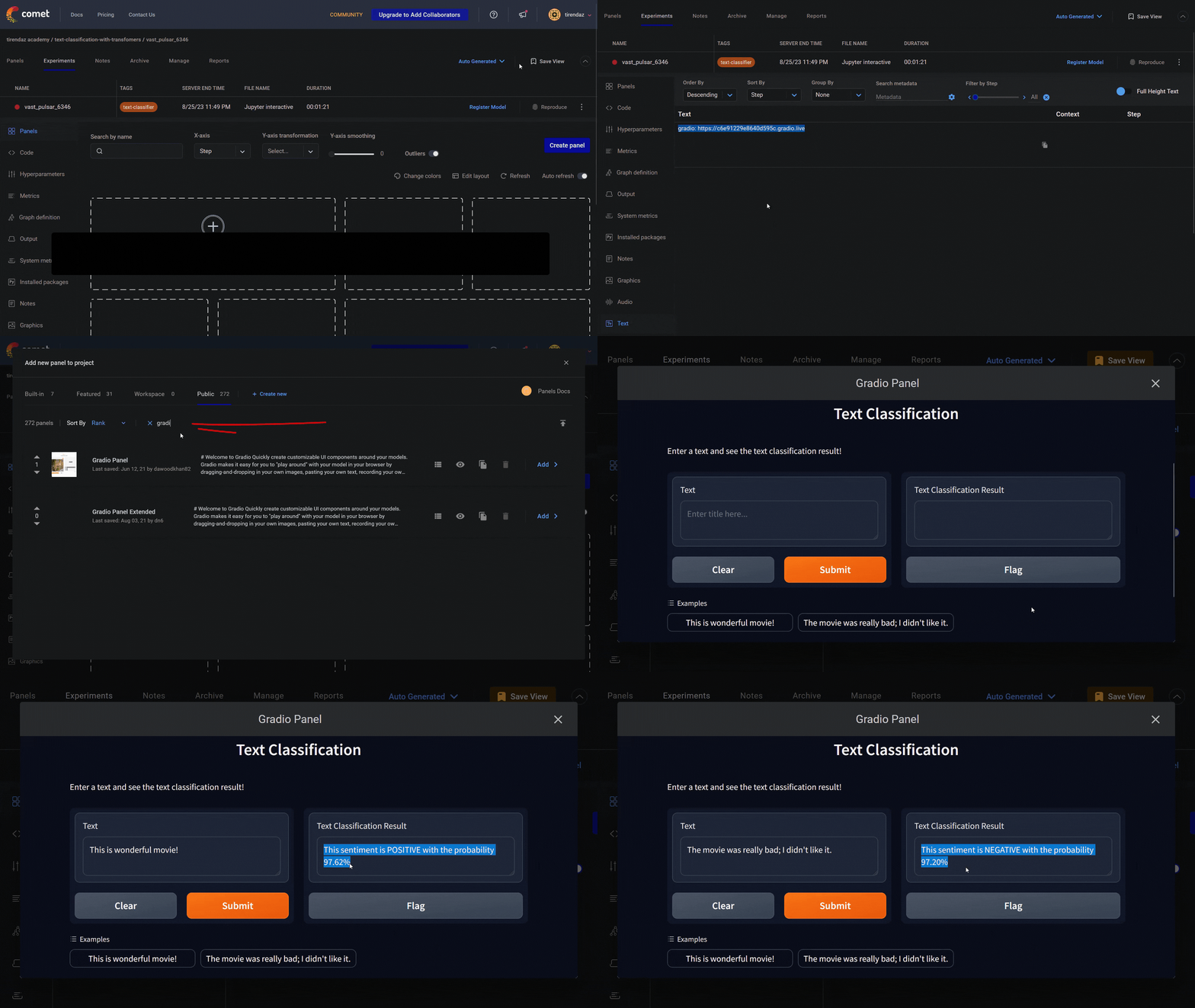
Great, we’ve built our web app. It’ll look like this in the Comet dashboard:

As you can see, we logged our Gradio app to Comet. We can now interact with it using the Gradio Custom Panel as above.

Wrap-Up

Congratulations, you now know how to build a BERT-based text classification app to classify the labels of texts. As you can see, this has become very easy with the recently developed platforms.

In this article, we first fine-tuned a BERT model with Transformers, built a Gradio app using this model, and then showcased it in the Comet dashboard.

That’s it. Thanks for reading. Let’s connect YouTube | Twitter | LinkedIn

If you enjoyed this article, please don’t forget to press the clap 👏 button below a few times 👇

Resources:

• Text Classification with Hugging Face
• Integrate with Hugging Face Transformers
• Natural Language Processing with Transformers