Using CLIP and Gradio to assess similarity between text prompts and ranges of colors
Hugging Face Space
Intro
OpenAI’s CLIP model and related techniques have taken the field of machine learning by storm since the group released their first blog post about the model in January 2021. I highly recommend that original post as an introduction to the big ideas of CLIP, if you haven’t read it already—but CLIP’s architecture and training process are outside the scope of this tutorial.
We’re going to focus on how to use the clip Python library to make similarity comparisons between text and images with pre-trained CLIP models. This basic functionality is at the heart of popular and highly sophisticated CLIP-based techniques. Notably, the model has been very popular in the AI art / generative images sphere, thanks to techniques originally made popular by artist and researcher Ryan Murdock. While the official CLIP repository provides a helpful Colab tutorial for “Interacting with CLIP,” this tutorial will start moving us toward using CLIP as a visual reasoning engine for generative work.
We’re going to use CLIP to compare individual solid colors to text prompts, and then see how our similarity score changes as we interpolate from one color to another.
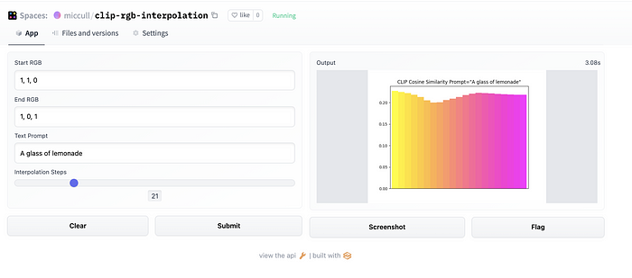
In the cover image for this blog post, for instance, I interpolated from a yellow (RGB=(1,1,0)) to a pink (RGB = (1,0,1)), and at each step, had CLIP report the similarity between that color and the phrase “A glass of lemonade.”
Higher scores denote greater similarity, so the bar chart tells us that the bright yellow is the best match for the text prompt. However, we see that as we fade from yellow to pink, some of the pink tones start to match “lemonade” very well, as well. It seems that the more bluish pinks closer to the right side of the plot start to get a little less similar to our text prompt.
We could imagine applying this idea toward optimizing a color. We provide a seed color—maybe a gray or a randomly generated RGB code—and we let CLIP guide us in adjusting that color to match it to a prompt as well as possible. We won’t do that in this tutorial, though. You’ll have to stay turned for part two of this series!
Prompt engineering plus Comet plus Gradio? What comes out is amazing AI-generated art! Take a closer look at our public logging project to see some of the amazing creations that have come out of this fun experiment.
Installing CLIP
Let’s go over installing CLIP first. The code shown below is intended for an IPython notebook, i.e. Colab. To run it in a bash shell, just remove the ! at the beginning of each line.
!pip install --quiet ftfy regex tqdm
!pip install --quiet git+https://github.com/openai/CLIP.git
Basics of working with CLIP
First, we need to load a pre-trained CLIP model. The clip library makes a number of models available, each corresponding to a slightly different architecture. Generally, there are two categories we’re dealing with: those models based on ResNet architectures and those based on VisualTransformer architectures.
# Should be one of ['RN50', 'RN101', 'RN50x4', 'RN50x16', 'ViT-B/32', 'ViT-B/16']
model_name = 'ViT-B/16'
model, preprocess = clip.load(model_name)# Set to "evaluation mode"
model.eval()
Encode some text
To encode text using a pre-trained CLIP model, there are a few things we need to do. The first is to tokenize the text as follows:
text = 'some text to encode'
tokenized_text = clip.tokenize(text)
Once the text is tokenized, it can be encoded using the pre-trained model’s text transformer.
encoded_text = model.encode_text(tokenized_text)
Images in PyTorch: Dimension Order
PyTorch adheres to a convention that may be unfamiliar if you’re used to working with images with PIL, NumPy, OpenCV, or TensorFlow. Say we have an RGB color image that is 640 pixels wide by 480 pixels tall. While PIL, NumPy, etc. would treat this as an array of shape (480, 640, 3), in PyTorch it would be (3, 480, 640).
This means that, if you load images using PIL, for instance, you must rearrange the dimensions to the proper order. This can be accomplished using the .permute() method for torch tensors. For example:
img = Image.open('/path/to/image.png')
arr = np.array(img)
# Rearrange the dimensions from (HWC) to (CHW)
x = torch.tensor(arr).permute((2,0,1))
But that’s not the whole story! If we had a stack of 10 images of this size, we would store them in a tensor of shape (10, 3, 480, 640). In other words, PyTorch formats images as (N, Channel, Height, Width) or NCHW. Moreover, many models are designed to work with batches of images, and you may need to convert a tensor of shape (C,H,W) to (1,C,H,W) . This can be accomplished using the .unsqueeze() method as follows:
# Old x.shape = (C, H, W), new x.shape will be (1, C, H, W)
# because .unsqueeze is expanding dimension 0
x = x.unsqueeze(0)# Similarly, we can do (?)
x = x.squeeze(0)
Encode an image
With CLIP, our goal is to make multi-modal comparisons — more specifically, we want to measure similarity across images and text. CLIP learns its image and text encoder models together, and we can access the image encoder via the .encode_image method of a trained CLIP model:
img = Image.open('/path/to/image.png')# We can just use the model's associated preprocesser function
x = model.preprocess(img)encoded_image = model.encode_image(x)
Encode a single color as an image
Of course, for our example in this tutorial, we’re not working with existing images. We’re generating our own!
Let’s write a function that turns a color in floating-point RGB space into a properly formatted image tensor. In other words, we may have something like color = (1, 0, 0) for red or color = (0.5, 0.5, 0.5) for a 50% gray. Really, this comes down to instantiating a tensor object and reshaping it to NCHW format. This function returns a 1×1 pixel image with RGB channels. More aptly, it outputs a stack containing a single image.
def create_rgb_tensor(color):
  """color is e.g. [1,0,0]"""
  return torch.tensor(color, device=DEVICE).reshape((1, 3, 1, 1))red_tensor = create_rgb_tensor((1, 0, 0))
But we can’t pass one of these into our visual encoder just yet. Recall that the CLIP model has a predefined resolution, which can be found with model.visual.input_resolution.
For us, this input resolution is a height and width of (224,224) . So let’s resize our RGB image. There are any number of ways we could do this using torch and torch-compatible libraries, but I’ll use the Resize class from torchvision.transforms.
from torchvision.transforms import Resize# Create the Resizer
resolution = model.visual.input_resolution
resizer = torchvision.transforms.Resize(size=(resolution, resolution))resized_tensor = resizer(red_tensor)torch.encode_image(resized_tensor)
Similarity
We now have encoded text and encoded images. How do we measure the similarity between them? We could employ any number of possible similarity metrics, but we’ll take cosine similarity as a starting point.
similarity = torch.cosine_similarity(encoded_text, encoded_image)
Create and interpolate between colors
We’re almost there…We can encode text. We can generate images from colors. We can resize those colors to the proper size for CLIP. And we can encode those images using CLIP.
Now, let’s write a function to interpolate between two colors. We’ll stick with linear interpolation, which simply “draws a line” between two endpoints. Note that the function below is called lerp which stands for (L)inear int(ERP)olation. This abbreviation is a strong convention, in my experience, and you’re likely to see it when and where you see a linear interpolation function defined in code.
def lerp(x, y, steps=11):
  """Linear interpolation between two tensors """

	weights = np.linspace(0, 1, steps)
	weights = torch.tensor(weights, device=DEVICE)
	weights = weights.reshape([-1, 1, 1, 1])

	interpolated = x * (1 - weights) + y * weights
  return interpolatedblue_tensor = create_rgb_tensor((0,0,1))
color_range = lerp(red_tensor, blue_tensor, 11)color_range = resizer(color_range)similarities = torch.cosine_similarity(encoded_text, color_range)
Plotting colors in Pandas

There are a few more functions we need for turning these colors into a nice bar plot in Pandas, but I won’t describe them all in detail here. Here’s a code snippet detailing this process:
def rgb2hex(rgb):
"""Utility function for converting a floating point RGB tensor to a hexadecimal color code."""
    rgb = (rgb * 255).astype(int)
    r,g,b = rgb
    return "#{:02x}{:02x}{:02x}".format(r,g,b)def get_interpolated_scores(x, y, encoded_text, steps=11):
  interpolated = lerp(x, y, steps)
  interpolated_encodings = model.encode_image(resizer(interpolated))  scores = torch.cosine_similarity(interpolated_encodings,
encoded_text)
  scores = sc.detach().cpu().numpy()  rgb = interpolated.detach().cpu().numpy().reshape(-1,  3)
  interpolated_hex = [rgb2hex(x) for x in rgb]    data = pd.DataFrame({
      'similarity': scores,
      'color': interpolated_hex
  }).reset_index().rename(columns={'index':'step'})  return datadef similarity_plot(data, text_prompt):
  title = f'CLIP Cosine Similarity Prompt="{text_prompt}"'
  fig, ax = plt.subplots()
  plot = data['similarity'].plot(kind='bar',
                                 ax=ax,
                                 stacked=True,
                                 title=title,
                                 color=data['color'],
                                 width=1.0,
                                 xlim=(0, 2),
                                 grid=False)
  plot.get_xaxis().set_visible(False) ;
  return fig
Deploying Our Model with Gradio and Hugging Face Spaces
We can get this process working in a Colab notebook, but let’s talk about deploying this model as an interactive app. I’ll be using Gradio as a framework and Hugging Face Spaces to deploy.
Gradio code
I won’t go into great detail about writing a Gradio app, but here are the basics:
- Define a function for the app to run. This is happening below with
gradio_fn. Note that this is just a Python function, and doesn’t actually require any Gradio specific stuff yet. This is simply what Gradio will do with the inputs we provide. - Define inputs for the Gradio interface. Gradio handles inputs using classes from the
gradio.inputsmodule. In this example, we’re usingTextboxinputs to write RGB values and aSliderto select the number of steps. Gradio’s simplicity is a big part of its appeal — the apps are not only simple to set up, but also have very uniform interfaces. There are other things that Gradio does an amazing job of handling for us, such as spinning up temporary, publicly shareable apps from a single line of code in a Colab notebook with no signup necessary! If we wanted to create something more custom, though—for instance if we wanted to use a color picker to select our RGB values—we might look at a framework like Streamlit. Streamlit is also supported by Hugging Face Spaces, and is overall excellent, but I went with Gradio this time, especially because it’s easy to test on Colab. - Create and launch the Gradio interface. We have a function to run, and we have input components for our interface, so now we just need to create a
gradio.Interfaceobject, which takes as arguments our function, inputs, and an output type. Then we simply call the.launch()method! As I mentioned before, what’s really amazing is that this method will work from a Colab cell, spitting out a public link and opening an inline IFrame with our app. But it will also work in our.pyfile on Hugging Face Spaces.
def gradio_fn(rgb_start, rgb_end, text_prompt, steps=11, grad_disabled=True):
  rgb_start = [float(x.strip()) for x in rgb_start.split(',')]
  rgb_end =  [float(x.strip()) for x in rgb_end.split(',')]  start = create_rgb_tensor(rgb_start)
  end = create_rgb_tensor(rgb_end)
  encoded_text = encode_text(text_prompt)
  data = get_interpolated_scores(start, end, encoded_text, steps)
  return similarity_plot(data, text_prompt)gradio_inputs = [gr.inputs.Textbox(lines=1, default="1, 0, 0", label="Start RGB"),
                 gr.inputs.Textbox(lines=1, default="0, 1, 0", label="End RGB"),
                 gr.inputs.Textbox(lines=1, label="Text Prompt", default='A solid red square'),
                 gr.inputs.Slider(minimum=1, maximum=30, step=1, default=11, label="Interpolation Steps")]iface = gr.Interface(fn=gradio_fn, inputs=gradio_inputs, outputs="plot")
iface.launch()
Next steps
What else can we do now that we can compare images and text using CLIP? The list is long, believe me, but here are some broad ideas:
- Zero-shot classification: In the vein of this project, we could imagine selecting from a predefined set of colors. For instance, selecting a Pantone color by providing a text prompt. This tutorial actually took us much of the way toward zero-shot classification. After computing the similarity score for every color in our set of interpolated colors, we would just need to report the “best match”.
- Directly modifying an image/text/some latent representation to maximize (or minimize) similarity. This is the basic idea driving many of the popular CLIP-enabled generative projects, such as CLIP+VQGAN (here’s a great read on VQGAN, by the way), CLIP Guided Diffusion, and CLIP+StyleGAN3. In fact, we can generalize here. We could take this process “in reverse” and use CLIP to generate captions by modifying a latent text representation to better match an image.
- Some projects take the CLIP+Generator idea to the next level. Look at researcher Mehdi Cherti’s “Feed forward VQGAN-CLIP model”, which uses CLIP and VQGAN to build a dataset of VQGAN’s responses to CLIP prompts, then performs supervised learning on that prompt/image dataset to learn to predict the latent space of VQGAN directly, bypassing the compute-heavy iterative process espoused by the standard CLIP+Generator approach.
Next in this series
Next time, we’ll look at using CLIP to guide the training of a PyTorch model to directly generate a color to best match a prompt. We’ll also start comparing aspects of the different pre-trained CLIP models in terms of performance and efficiency, and we’ll look at how to track the parameters and outputs of runs with Comet.