“Text-to-Color” from Scratch with CLIP, PyTorch, and Hugging Face Spaces
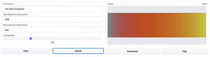
Example input and output from the Gradio app built using the Text to Color model. Moving from left to right, we can see how each progressive training step updates the color to match the prompt “the color of a banana”.
Introduction
This is part two in a series on using CLIP from scratch to evaluate and manipulate images by comparing them to text prompts. Part one can be found here.
In the last post, I demonstrated how to compare a text prompt across a range of colors and visualize how well each individual shade matched the text prompt. In this tutorial, I’ll demonstrate how we can optimize a color to match text as well as possible. To do so, we’ll write a custom Module using PyTorch.
You can follow this Colab notebook to work with the code interactively, and you can also try the model in action at this Hugging Face Space, which I built using Gradio. In this post, I’ll provide some commentary and explanation on the code needed to write the model and training loop.
Subclass from torch.nn.Module:
The first thing we do is create a new class, RGBModel, as a subclass of PyTorch’s Module class. If you’re not familiar with the idea of classes and inheritance in Python (or another language), this is like creating our own recipe for a model by adapting from some fundamental building blocks.
The Module class takes care of a lot of low-level functionality in PyTorch, and we just add a few custom things on top of it.
class RGBModel(torch.nn.Module):
    pass
Define __init__ method:
First, we need to define our initializer, which gets called whenever we create a new instance of this class, i.e. when we write something like model = RGBModel().
class RGBModel(torch.nn.Module):
    def __init__(self, device):
      # Call nn.Module.__init__() to instantiate typical torch.nn.Module stuff
      super(RGBModel, self).__init__()
			color = torch.ones(size=(1,3,1,1), device=device) / 2
      self.color = torch.nn.Parameter(color)
The first thing our __init__ method does is call the standard __init__ method from torch.nn.Module, which is our “parent” class or superclass. That’s what super(RGBModel, self).__init__() is doing. That handles all sorts of standard PyTorch initialization stuff that we need to get off the ground.
Then, we define a Parameter for our model. This will hold the RGB value that we optimize in the training loop. We first create a tensor of all ones, and of shape (1,3,1,1), using torch.ones. Remember that PyTorch typically expects images in the NCHW format. So that means we’re setting our tensor up as a stack of images containing one RGB image with a width and height of a single pixel. We could handle reshaping this parameter later, but this will be more convenient for us downstream when the time comes to resize the pixel to the input resolution for CLIP’s image encoder.
Next, we pass this tensor into the torch.nn.Parameter and store this object as an attribute. That way, it will persist over time and we can access it via other methods.
Define forward pass:
class RGBModel(torch.nn.Module):
    def __init__(self, device):
      # Call nn.Module.__init__() to instantiate typical torch.nn.Module stuff
      super(RGBModel, self).__init__()
			color = torch.ones(size=(1,3,1,1), device=device) / 2
      self.color = torch.nn.Parameter(color)    def forward(self):
      # Clamp numbers to the closed interval [0,1]
      self.color.data = self.color.data.clamp(0,1)      return self.color
Next, we define what the model actually does when it’s called. If __init__ is what happens when we write model = RGBModel(), then forward dictates what happens when we then call model(). We might think of this as a “prediction” or “generation” step, in many cases, but ultimately this is what the model actually outputs.
For us, the forward pass is quite simple. The model should simply output its color. We do not want forward to handle turning that color into an image or anything like that. The only thing we need to do is ensure that our color stays within an appropriate range during the training process. As such, we’re writing self.color.data = self.color.data.clamp(0, 1) to restrict our model to the closed interval [0, 1].
There are some issues we could run into with the clamp method during training, but this is a toy model, so we’re going to ignore that for now.
Want to see the evolution of AI-generated art projects? Visit our public project to see time-lapses, experiment evolutions, and more!
Create an Optimizer
With our model ready to go, it’s time to create an optimizer object. We’ll use the AdamW optimizer. For more information, this blog post is a great rundown of the AdamW algorithm and its predecessor, Adam.
# Create optimizer
opt = torch.optim.AdamW([rgb_model()],
											   r=adam_learning_rate,
												 weight_decay=adam_weight_decay)
Basically, what we need to know is that AdamW defines a strategy for running incremental, iterative updates to our color parameter during the training process.
Here, we provide two hyperparameters to the optimizer when we create it: a learning rate and a weight decay value. Broadly speaking, the learning rate describes the magnitude of updates each training step should make (higher rate = bigger increments), and the weight decay drives a process by which those update steps shrink over time.
In the context of our model, the optimizer will help tell us something like “if you want to make your color match this prompt, you should turn up the red value.” Or more specifically, it would tell us something like “if you add something to your color in the direction of, say, (0.1, -0.1, 0.1) , it would increase the similarity the fastest.” Then, the learning rate comes into play by modifying how large that increment is. Over time, we want to take smaller, more precise steps, so the optimizer implements weight decay to do just that.
Generate a Target Embedding
We have a model and an optimizer. What do we optimize towards? Let’s set up our target.
# Create target embedding
with torch.no_grad():
    tokenized_text = clip.tokenize(text_prompt).to(device=DEVICE)
    target_embedding = model.encode_text(tokenized_text).detach().clone()
This should look familiar if you’ve read part one of this series. But I want to point out an optional step we’ve taken here by computing this encoded text using a torch.no_grad context handler. What’s that all about?
Basically, PyTorch and other deep learning libraries use something called automatic differentiation to keep track of the gradients/derivatives of tensors as they move through a computational graph. Automatic differentiation simplifies a lot of computation when necessary, but it uses more memory in the process.
We absolutely need this to be enabled for the color parameter of our RGBModel, since we need to compute the gradient of the (not yet defined) loss function to update the color during training. However, we don’t need to take the gradient of anything with respect to our target, so we can save some memory by creating it in an indented block under with torch.no_grad().
For a model this simple, we almost surely are not that concerned with how much memory we have, but it will be a helpful trick in future projects when we start pushing the limits of our machines.
Define the Training Step
Now, we define the actual training process. What happens during each iteration of our training loop? At the heart of it, we need to encode our color as an image, then compare its CLIP embedding to the embedding for our text prompt. But there are a few more things going on in here that you may or may not have seen before.
def training_step():
	# Clear out any existing gradients
  opt.zero_grad()

	# Get color parameters from rgb model instance
	color = rgb_model()
  color_img = resizer(color)
  image_embedding = model.encode_image(color_img)

	# Using negative cosine similarity as loss
	loss = -1 * torch.cosine_similarity(target_embedding, image_embedding, dim=-1)

  # Compute the gradient of the loss function and backpropagate to other tensors
	loss.backward()  # Perform parameter update on parameters defined in optimizer
	opt.step()
Notes: opt.zero_grad()
We want to compute the gradient for each step of the training loop separately, which is the standard way of doing things, but not the only way. It turns out that PyTorch optimizers store or accumulate gradients until we flush those values out with opt.zero_grad().
It may seem like this step should be automatic after performing an update, but there are many techniques that benefit from accumulating gradients. Making this process manual in PyTorch gives us lots of transparency and flexibility in defining how models train.
Notes: loss.backward()
We compute our loss tensor loss as the negative cosine similarity between the CLIP embeddings of our text prompt and of our model’s current color parameter. With loss functions, we want something where smaller is better, which is why we’re using the negative cosine similarity.
Once we compute the loss, we need to compute its gradient. Don’t be fooled; despite the term “automatic differentiation,” this doesn’t actually happen automatically!
Automatic differentiation refers to the accumulation of symbolic steps that can be combined using the chain rule to produce the gradient of a function/tensor. Thus, calling loss.backward() will compute the gradient with respect to the graph’s leaves (in this case, the color parameter of our model) so the optimizer can use it.
Notes: opt.step()
So now we have our loss, and we’ve computed its gradient with respect to color. It’s time we updated our color. Calling opt.step() will do just that. If we leave this out, then color will never change.
What’s Next?
In this post, we used CLIP to drive the direct optimization of RGB values to match text prompts. Along the way, we covered some PyTorch fundamentals, working with the Module class to create models and unpacking some aspects of the training process. How do we build from here?
We could iterate on this work in any number of ways. For one, we could move to optimizing more than one pixel at a time. Maybe we try to directly optimize an 8×8 RGB image with CLIP. If we simply use CLIP-driven cosine similarity as our loss function, we will find that we get increasingly unstable results if we just try to optimize pixel values directly. Instead, we could try swapping our RGBModel with another image-generating mechanism. For instance, we could use the generator from a GAN, and use CLIP to optimize the latent vectors, implicitly capturing changes in features that extend beyond individual pixels. In fact, that appears to be the most popular approach in CLIP-guided image generation. Not sure what all of that means? Then stay tuned to learn more in the next installation in this series.
For now, you can try this model live on Hugging Face Spaces, and also read through the code that drives the demo. You can also find out more about Hugging Face and Gradio here.