Fraud Detection, Imbalanced Classification, and Managing Your Machine Learning Experiments Using Comet

An end-to-end guide for building and managing an ML-powered fraud detection system
A brief history of fraud
The earliest recorded attempt of fraud can be found as far back as the year 300 BC in Greece.
A Greek sea merchant named Hegestratos sought to insure his ship and cargo, so took out an insurance policy against them. At the time, the policy was known as a `bottomry` and worked on the basis that a merchant borrowed money to the value of his ship and cargo.
As long as the ship arrived safe and sound at its destination with its cargo intact, then the loan was paid back with interest. If on safe delivery the loan was not repaid, the boat and its cargo were repossessed.
Hegestratos planned to sink his empty boat, keep the loan, and sell the corn. The plan failed, and he drowned trying to escape his crew and passengers when they caught him in the act.

Some 2,000+ years later financial institutions are still fighting the same battle.
Machine learning and fraud
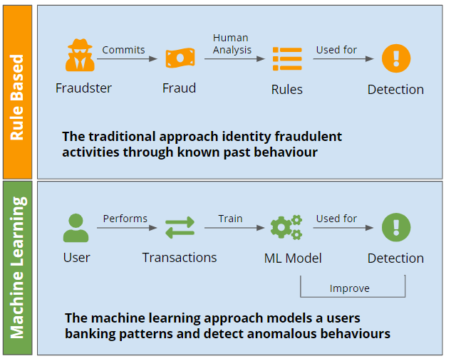
Traditionally, financial institutions automatically flagged transactions as “high risk” based on a set of clearly defined rules, and then either denied or manually reviewed flagged transactions.
While these rules-based systems are still an important part of the anti-fraud toolkit, they were never designed for modern internet businesses.
This new era of finance and banking has seen tremendous innovation from companies such as PayPal, Stripe, Square, and Venmo which have made it easy for any one to send and receive money right from their phones.
This has led to many financial institutions being flooded by a tsunami of data.
Machine learning algorithms capable of processing these ever increasingly large datasets have been an indispensable in helping financial institutions identify correlations between user behavior and the likelihood of fraudulent actions.
Data scientists have been successful in authenticating transactions using machine learning and predictive analytics.
Automated fraud screening systems powered by machine learning can swiftly and accurately detect a fraudulent transaction, mitigating the risk of that transaction going through and saving financial intuitions and their customers millions of dollars.
Problem statement
Imagine yourself as a data scientist at a company that builds products which enable millions of small e-commerce merchants and small, local business owners to conduct business online.
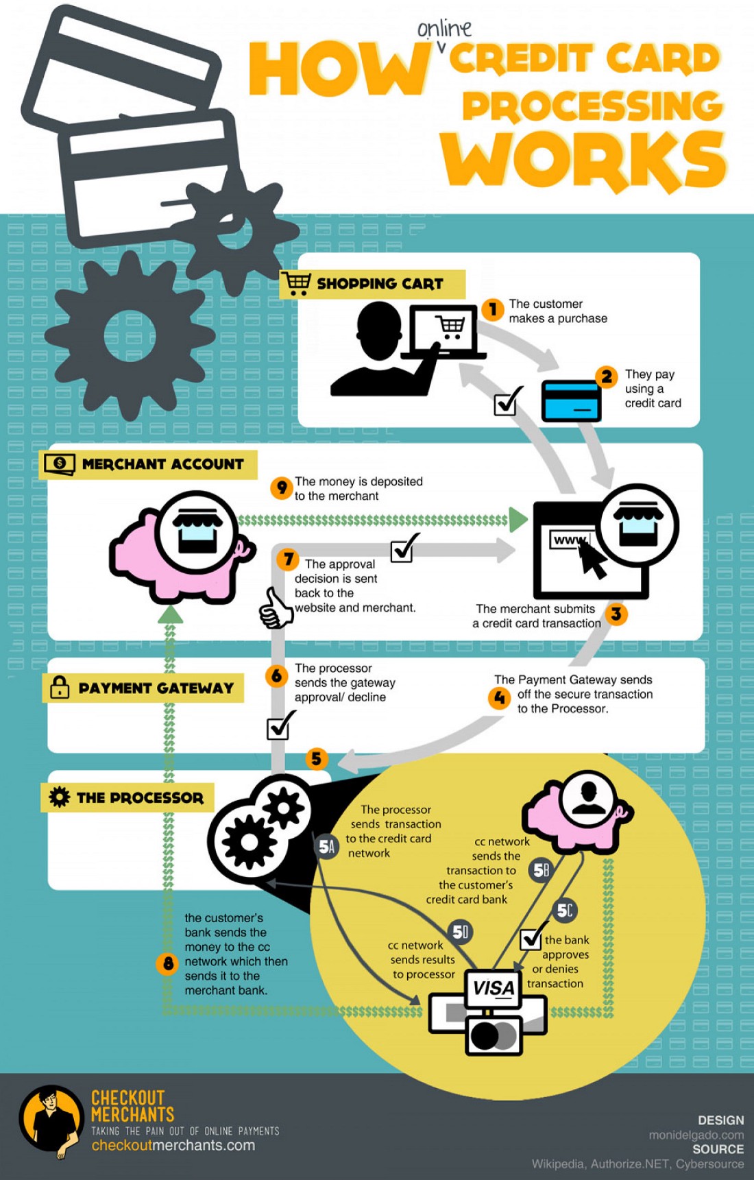
Unlike the brick-and-mortar counterparts, online merchants are held liable for fraudulent purchases.
When a cardholder’s bank declares a transaction as fraudulent, the cardholder is fully reimbursed while the merchant is left footing the cost of the fraud.
This cost is always more than just the dollar amount of the transaction, because not only do they lose the value of the item sold — whatever it cost them to make it or purchase it themselves — they’re also responsible for any fees resulting from the dispute.
These costs can add up and have a significant negative impact on these merchants livelihoods.
Your company wants to help merchants focus on their product and customer experiences — and not on fraud — so they’re developing a suite of modern tools for fraud detection and prevention.
Central to which is a machine learning model which evaluates transactions for fraud risk and takes action appropriately.
Using the dataset provided, your task is to build a machine learning model which provides greatest protection against fraudulent transactions by correctly classifying and blocking fraudulent transactions.
Data
Here’s some high level details about the dataset we’re working with:
- We have a highly imbalanced dataset, with 99% of transactions being legitimate and less than 1% (n = 8,213) being fraudulent.
- All fraudulent transactions come from
CASH_OUT(n = 4,116) andTRANSFER(n = 4,097) type transactions.TRANSFERis where money is sent to a customer / fraudster andCASH_OUTis where money is sent to a merchant who pays the customer / fraudster in cash. Speaking to stakeholders we identify that the modus operandi for fraudulent transactions: fraud is committed by first transferring out funds to another account which subsequently cashes it out. - 6.3 million transactions coming with 2.7 million unique values for the feature
nameDest, which is the feature indicating recipient id of the transaction. Speaking to the stakeholders learn that the naming scheme for bothnameDestandnameOrigcolumns is as follows: IDs beginning withCindicate it is a customer account, and IDs beginning withMindicate it is a merchant account.
And here are the features present in our data set:
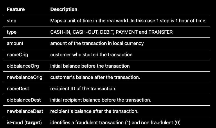
Note, this data is actually simulated data from the PaySim Kaggle Competition. You can visit the source by following this link:
The challenge in building a model
In any binary classification problem — such as the one we’ve got here — there are two types of misclassifications we can make: False positives and false negatives
And the main challenge here is: how do we tell if our model is any good?
Let’s explore this a bit deeper.
False negatives
These are instances of fraud which are not identified or prevented before a dispute occurs, when your model says a transaction is not fraudulent but it really is.
False positives
These are legitimate transactions which are blocked by a fraud detection system, when your model says a transaction is fraudulent but it really isn’t.
The tradeoff
A tradeoff exists between false negatives and false positives.
Optimize for fewer false negatives, and you must be willing to tolerate a greater occurrence of false positives (and vice versa).
A false negative incurs the cost of goods sold and the fee for disputes. A false positive incurs the margin on the goods sold.
Businesses need to decide how to trade off the two.
So, which do you choose to optimize for?
When a business has small margins, the false negative is a more costly mistake to make than a false positive. In this case, we would want to be more robust and try to stop as many potentially fraudulent cases as possible. Even if it means more false positives.
The opposites is true when margins are larger: false positives become more costly than false negatives.
The data scientist faces the problem of building a good machine learning model by engineering the right features and finding the best algorithm for their business, and the business problem of picking a policy for actioning a given machine learning model’s outputs.
The business policy
Suppose that our business prescribes policy to block a payment if the machine learning model assigns the transaction a probability of being fraudulent of at least 0.8 — in math terms P(fraud) >= 0.8.
This is because from the businesses point of view we want to be fairly confident before we block a transaction, because it can be a nuisance to merchants if they have too many non-fraudulent transactions flagged as fraudulent. This situation would cause a poor user experience and result in unhappy customers.
Evaluating the machine learning model
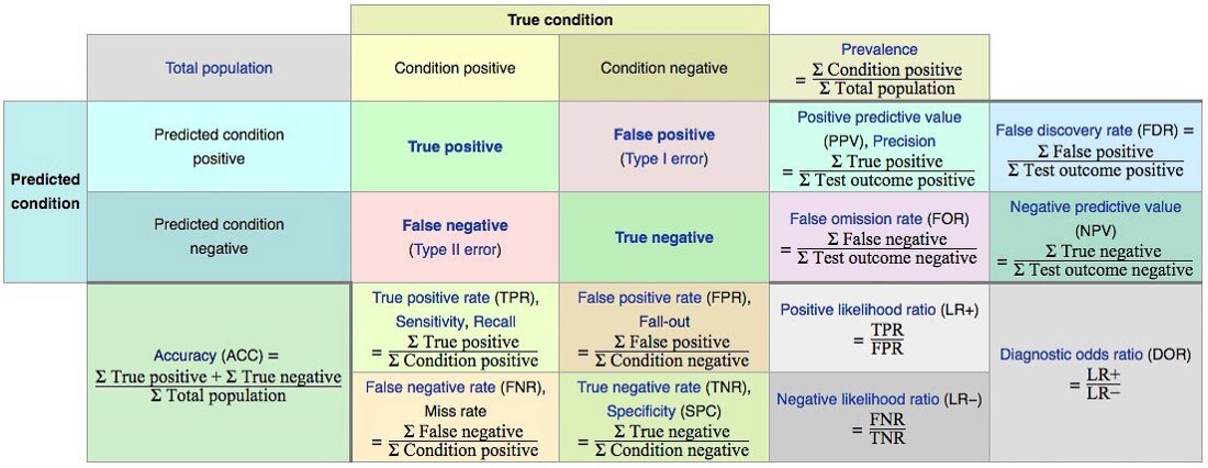
There are A LOT of metrics we can choose to evaluate our machine learning model.
A simple confusion matrix yields 14 metrics.
Let’s examine three of these in closer detail: precision, recall, and false positive rate.
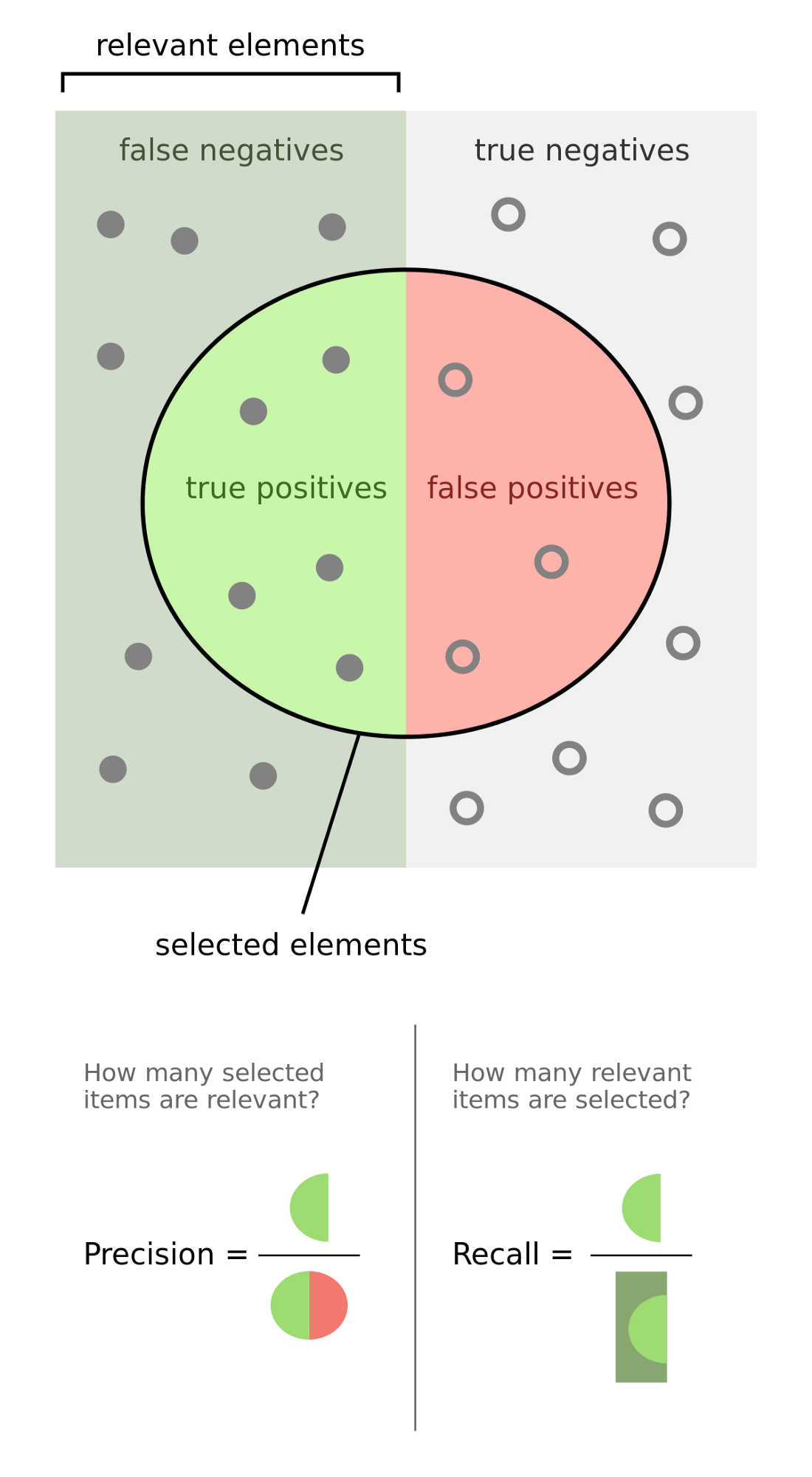
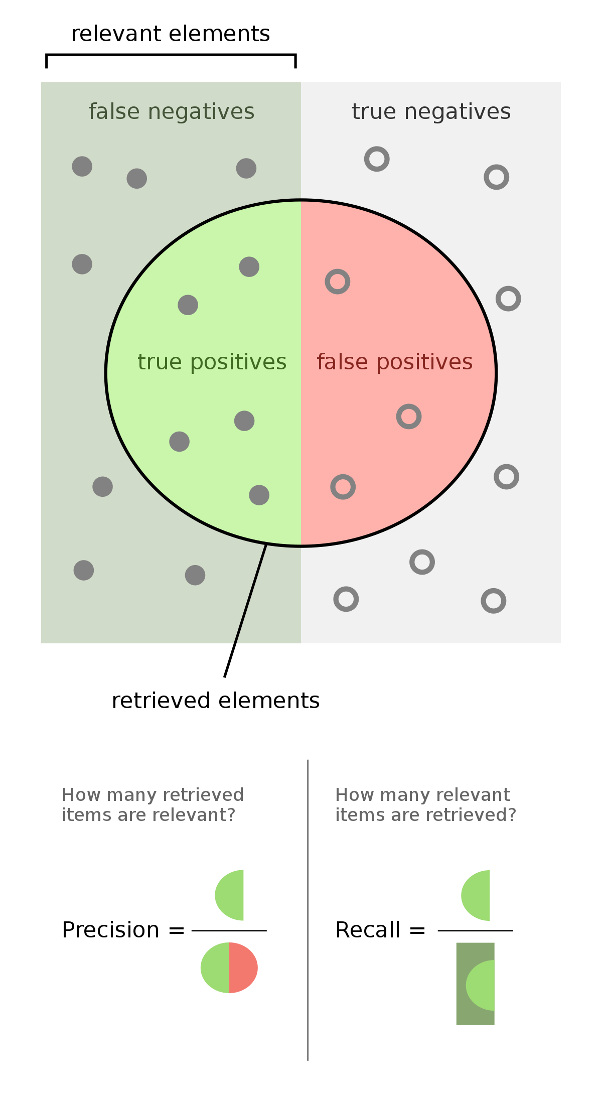
Precision
The precision of our model is the proportion of transactions our model flagged as fraudulent which are truly fraudulent.
Example: Suppose we had 100 transactions, and our model flags 60 of these as fraudulent.
And of those 60 transaction that were flagged as fraudulent, 40 are actually fraudulent.
Then the precision would be 40 / 60 = 0.66.
A higher precision implies a fewer number of false positives.
Recall
The recall of our model (aka true positive rate) is the proportion of all truly fraudulent transactions which were flagged as fraudulent by our model.
Example: Suppose we had 100 transactions, and 50 of these are truly fraudulent.
And of these 50 truly fraudulent transactions, our model flags 40 of them as fraudulent.
Then the recall is 40 / 50 = 0.8.
A higher implies recall implies a fewer number of false negatives.
False positive rate
The false positive rate of our model is the proportion of all legit (non-fraudulent) transactions which the model incorrectly flagged as fraudulent.
Example: Suppose we had 100 transactions, and 50 of these are transactions are legit.
And of these 50 legit transactions, our model flagged 20 of them as fraudulent.
Then the false positive rate is 20 / 50 = 0.4.
So you’re probably wondering…What are “good values” for precision, recall, and false positive rate.
If we had a perfectly clairvoyant model, then 100% of of the transactions it classifies as fraud would actually be fraud.
This would imply a few things about the values of precision, recall, and false positive rate:
- Precision would equal 1 (100% of transactions that the model classifies as fraud are actually fraud).
- Recall would equal 1 (100% of actual fraud cases are identified).
- False positive rate would equal 0 (no legitimate transactions were incorrectly classified as fraudulent).
We don’t often build clairvoyant models, so there is a tradeoff between precision and recall.
The impact of the probability threshold
As we increase the probability threshold for blocking (the business policy we discussed earlier), precision will increase.
That’s because the criterion for blocking a transaction is more strict, which implies a high level of “confidence” for classifying the transaction as fraudulent. This, in turn, results in fewer false positives.
By the same logic, it follows that increasing the probability threshold will cause recall to decrease, implying fewer false negatives. That’s because we now have fewer transactions match the high probability threshold.
Conversely, when we decrease the probability threshold the reverse happens: precision will decrease and recall will increase.
ROC and precision-recall curves
ROC Curves
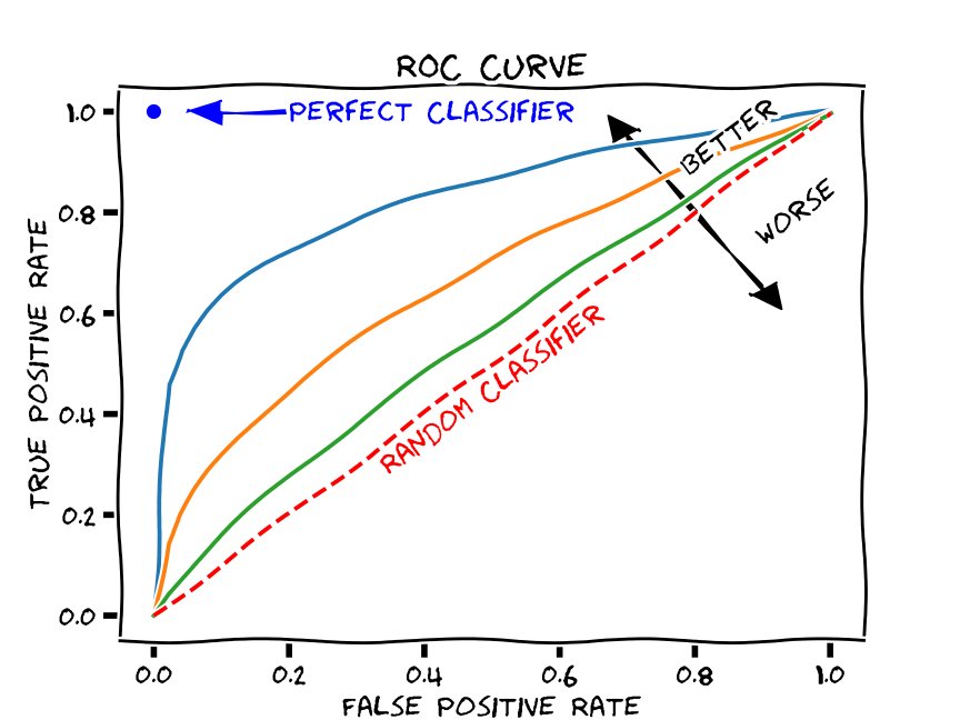
One way to understand and visualize this trade-off is through the ROC-curve, which plots recall (aka true positive rate) against the false positive rate
A perfect model will have an ROC curve that hug the top left of the graph — where recall is 1.0 and the false positive rate is 0.0.
A random model would have the true positive rate equal the false positive rate, and we’d end up with a straight line.
We hope to build a model that’s somewhere between a perfect model and a random guesser.
One way to capture the overall quality of the model is by computing the area under the curve ROC curve (ROC AUC).
Class imbalance changes everything
When the classification problem becomes an imbalanced classification problem — the ROC AUC becomes misleading.
This imbalanced situations a small number of correct or incorrect predictions can result in a large change in the ROC Curve or ROC AUC score.
A common alternative is the precision-recall curve and area under curve.
Precision-recall curves
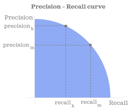
A precision-recall curve (or PR Curve) is a plot of the precision (y-axis) and the recall (x-axis) for different probability thresholds.
A perfectly skilled, clairvoyant model would be depicted as a point at a coordinate of (1,1).
A random, no-skill classifier will be a horizontal line on the plot with a precision that is proportional to the number of fraudulent transactions in the dataset.
As a model becomes better and better the it will start to hug the top-right of the graph — where precision and recall are both maximized at 1.0.
Because the Precision-Recall curve puts more emphasis on the minority class, it proves to be an effective diagnostic for imbalanced binary classification models.
Just like with the ROC Curve, we can capture the overall quality of the model by computing the area under the precision-recall curve (PR AUC).
In our example, we’ll use the area under the Precision-Recall curve as an evaluation metric.
Methodology
Using the data provided by our stakeholders, we’ll perform some basic data understanding, exploratory data analysis, engineer features, balance our dataset, spot check candidate models, choose the best candidates for further hyper-parameter tuning, and finally evaluate models to identify which one we’ll add to our model registry.
Each of the notebooks linked below has all the details for each step in the methodology.
We’ll be tracking our experiments using Comet throughout!
Dependencies
We’ll use the following libraries in python to assist us with this project:
- pandas
- numpy
- scikit-learn
- imblearn
- Comet ML
- pycaret
- sweetviz
Notebooks
I firmly believe the best way to learn something is by trying it for yourself. Instead of just sharing code snippets, I thought it would be more fun for you to get hands on, so I’ve shared runnable Colab Notebooks so you can more easily follow along.
Fetch raw data

In this notebook we access the data provided to us by our stakeholders and log the raw data to Comet as an Artifact.
Data understanding

Profiling data using the sweetviz library to get a feel of it and see what’s going on in there. If you haven’t seen sweetviz in action, prepared to be impressed! It’s an an open-source Python library that generates beautiful, high-density visualizations to kickstart EDA (Exploratory Data Analysis) with just two lines of code.
Learn more about how sweetviz integrated with Comet here:
Exploratory data analysis and feature engineering

More in-depth analysis of the data and creating new features from raw data. We’ll also log versions of our data as an Artifact to Comet to keep track of it.
Spot-checking algorithms

We’ll spot-check a suite of classification algorithms and choose the best one for further hyper-parameter tuning.
Experimenting with hyper-parameters

We’ll use Comet to run experiments and select the best combination of hyper-parameters for these algorithms.
We’ll then evaluate the performance on the test set and register it on the Model Registry in Comet. This is an incredibly useful tool which allows us to store trained machine learning models, metadata about the data and training jobs used to create the model, and keep track of which versions are in production. This is a critical piece of the puzzle for establishing lineage for ML models.
Conclusion
That’s it! I hope you’re ready to explore the notebooks, run them for yourself, and see what the end-to-end process we’ve outlined in this post looks like.
I’ve also included some homework for you within the notebooks! Machine learning is an art as much as a science, and the art comes from the various ways you can experiment with the process.
I’ve included some suggestions in each of the notebooks for things that you can try on your own, and my hope is that you come up with some interesting ideas and share them with me in our open Slack community.
That’s it for this write up, I’ll see you in the notebooks.
And remember my friends: You’ve got one life on this planet, why not try to do something big?
Related Articles