The Gradient Descent Algorithm

Gradient descent is one of the most used optimization algorithms in machine learning. It’s highly likely you’ll come across it so it’s worth taking the time to study its inner workings. For starters: optimization is the task of minimizing or maximizing an objective function.

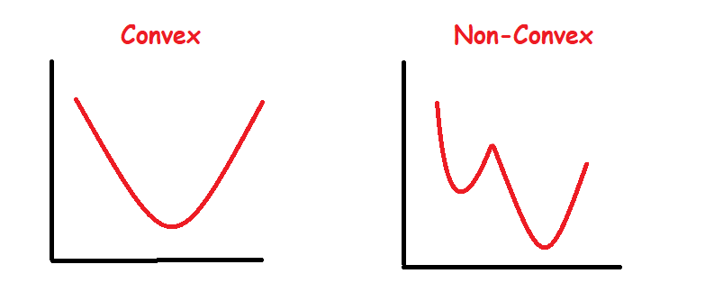
Typically we’d prefer to minimize the objective function in a machine learning context and gradient descent is a computationally efficient way to do so. This means we want to find the global minimum of the objective function but we can only achieve that goal if the objective function is convex. In the event of a non-convex objective function, settling with the lowest possible value within the neighborhood is a reasonable solution. This is usually the case in deep learning problems.

How are we performing?

Before we start wandering around, it’s good to know how we’re performing. We use a loss function to work this out. You may also hear people refer to it as an objective function (the most general term for any function that’s being optimized), or cost function.

Most people wouldn’t be bothered if you used the terms interchangeably but the math police would probably pull you up — learn more about the differences between objective, cost, and loss functions. We will refer to our objective function as the loss function.

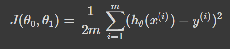
The responsibility of the loss function is to measure the performance of the model. It tells us where we currently stand. More formally, the goal of computing the loss function is to quantify the error between the predictions and the actual label.

Here’s the definition of a loss function from Wikipedia:

“A function that maps an event or values of one or more variables onto a real number intuitively representing some “cost” associated with the event. An optimization problem seeks to minimize a loss function.”

To recap: our machine learning model approximates a target function so we can make predictions. We then use those predictions to calculate the loss of the model — or how wrong the model is. The mathematical expression for this can be seen below.

What direction shall we move?

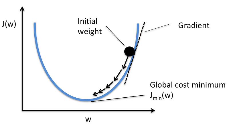
In case you’re wondering how gradient descent finds the initial parameter of the model, they’re initialized randomly. This means we start at some random point on a hill and our job is to find our way to the lowest point.

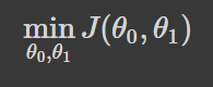
To put it technically, the goal of gradient descent is to minimize the loss J(θ) where θ is the model parameters.

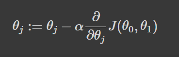
We achieve this by taking steps proportional to the negative of the gradient at the current point.

We’ve calculated the loss for the model. For our gradient descent algorithm to determine the direction that will permit it to converge fastest, the partial derivative of the loss is calculated. This is a concept from calculus that is used to reference the slope of a function at a given point. If we know the slope then we can figure out what direction to move in order to reduce the loss on the next step.

Most projects fail before they get to production. Check out our free ebook to learn how to implement an MLOps lifecycle to better monitor, train, and deploy your machine learning models to increase output and iteration.

How big shall the step be?

Among all the funny symbols in the equation above is a cute α symbol. That’s alpha, but we can also call her the learning rate. Alpha’s job is to determine how quickly we should move towards the minimum. Big steps would move us quicker and little steps will move us slower.

Figure 2: Example of minimizing J(w); (Source: MLextend)

Being too conservative, or selecting an alpha value that’s too small, is going to take longer to converge at the minimum. Another way to think of it is that learning will happen slower.

But being too optimistic, or selecting an alpha value that’s too large, is risky too. We can completely overshoot the minimum, thus increasing the error of the model.

The value we select for alpha has to be just right so we can learn fast, but not so fast that we miss the minimum. To do this we must find the optimal value for alpha such that gradient descent converges fast. This will require hyperparameter optimization.

Gradient Descent in Python

The steps to implement gradient descent are as follows:

1. Randomly initialize weights
2. Calculate the loss
3. Make a step by updating the gradients
4. Repeat until gradient descent converges.

def gradient_descent(X, y, params, alpha, n_iter): 
    """
    Gradient descent to minimize cost function
    __________________ 
    Input(s)
    X: Training data
    y: Labels
    params: Dictionary contatining random coefficients
    alpha: Model learning rate
    __________________
    Output(s)
    params: Dictionary containing optimized coefficients
    """
    W = params["W"] 
    b = params["b"]
    m = X.shape[0] # number of training instances 

    for _ in range(n_iter): 
        # prediction with random weights
        y_pred = np.dot(X, W) + b
        # taking the partial derivative of coefficients
        dW = (2/m) * np.dot(X.T, (y_pred - y)) 
        db = (2/m) * np.sum(y_pred -  y)
        # updates to coefficients
        W -= alpha * dW
        b -= alpha * db 
    
    params["W"] = W
    params["b"] = b
    return params

Several different adaptations could be made to gradient descent to make it run more efficiently in different scenarios — like when the dataset is huge. Have a read of my other article on Gradient Descent in which I cover some of the various adaptions as well as their pros and cons.

Thanks for reading.