We face optimization problems all the time in our daily life: you don’t merely pick up a random pair of jeans and head to the checkout when you’re doing clothes shopping — hopefully not, I should say. There’s a process to it:
You may want a specific brand of jeans.
Maybe dark-wash jeans are your go-to.
Maybe you have a certain fit you prefer: straight, slim, skinny.
Most important of all, the jeans have got to fit you — is your size available?
To feel like you’ve got your money’s worth, as you sift through the in-store jeans, you’re mentally recording whether they meet the criteria for the type of jeans you want to purchase.
The best jeans for you would mark all of your criteria (i.e. Levi branded, dark wash, stretch skinny fit, and your size) — those are the optimal jeans.
Let’s see what this optimization means in a machine learning context.
In this article we are going to discover the following, using Comet’s experiment management platform:
→ What it means to optimize a learning algorithm
→ Comet’s Optimizer class
→ Optimization approaches
→ An End-to-end example
Do you prefer to watch this tutorial? See Hyperparameter optimization with CometML
Optimizing learning algorithms
The hyperparameter optimization problem we face in machine learning is not too dissimilar from the one we face when out jeans shopping (or whatever we want to optimize for).
In the same way we’d search through various jeans, we need to search through various algorithms we wish to use to solve a problem at hand. Once we feel as though we’re onto something with a certain algorithm, it’s important to optimize the algorithm, which means we minimize the error to ensure the model is solving the problem to the best of its abilities — we’re “getting our money’s worth!”
Hyperparameters are values that control the learning process of an algorithm. When implementing a learning algorithm, we define these values beforehand, as there is no way for the algorithm to learn them from training. Examples of hyperparameters include:
- the number of trees in a random forest
- the learning rate of an algorithm
- the number of layers in a neural network
Implementing the optimal version of an algorithm means selecting the hyperparameters that minimize the error for the problem at hand —or put another way, we are trying to maximize the performance of our algorithm for the dataset being used.
When you begin on a problem, there is no clear way to know what hyperparameters will result in the optimal model. To find them we must do hyperparameter optimization.
Optimization with Comet
Comet is a machine learning platform that permits data scientists and teams to track, monitor, compare, explain, and optimize experiments as well as models. The optimizer will be our main focus in this article.
In line with Comet’s documentation, the Optimizer class may be used to:
“dynamically find the best set of hyperparameter values that will minimize or maximize a particular metric.”
The class is also capable of making suggestions as to what hyperparameter values may be worth trying next — which is done in serial, parallel, or a combination of both.
Arguments used to define the Optimizer include:
→ config: optional, if COMET_OPTIMIZER_ID is configured, otherwise is either a config dictionary, optimizer id, or a config filename.
→ trials: int(optional, default 1) number of trials per parameter set to test
→ verbose: boolean (optional, default 1) verbosity level where 0 means no output, and 1 (or greater) means to show more detail.
→ experiment_class: string or callable (optional, default None), class to use (for example, OfflineExperiment).
Notice there’s an option to pass a configuration dictionary to the config parameter. This is where we detail the optimization approach we want the Optimizer to perform.
The dictionary the config parameter wants us to pass consists of the following keys:
→ algorithm: string, the search algorithm to be used
→ spec: dictionary, the algorithm-specific specifications.
→ parameters: dictionary, the parameter distribution space descriptions
→ name: string, a distinct name to associate with the search instance (optional)
→ trials: integer, the number of trials per experiment to run (optional, defaults to 1).
Note: We will cover the various algorithms and their
specin the Optimization methods section.
The parameters dictionary is where we define what hyperparameters to tune in our model. Let’s take a closer look at what it consists of.
The Parameters dictionary
In our configuration dictionary, we have a parameters key, which takes a dictionary. In our parameters dictionary, we must define specific data types that are in accord with the data type our model hyperparameter is expecting.
Comet provides us with four types: 1) integer 2) double or float 3) discrete (for a list of numbers) 4) categorical (for a list of strings). The formatting of each parameter is inspired by Google’s Vizier. Let’s dive deeper into each one.
Integer and Double/Float
Integers and double/float types allow us to determine the scaling type of our values. Comet provides five possible distributions to select from: linear, uniform, normal, log uniform, log normal.
The scaling type we use determines the distribution between the min and max values of the hyperparameter.
{"PARAMETER-NAME":
   {"type": "integer",
   "scalingType": "linear" | "uniform" | "normal" | "loguniform" | "lognormal",
   "min": INTEGER,
   "max": INTEGER
   },
 ....
}
For clarity, the definitions are as follows:
→ linear: for integers, this means an independent distribution (used for things like seed values); for double, the same as uniform
→ uniform: a uniform distribution between “min” and “max”
→ normal: a normal distribution centered on “mu”, with a standard deviation of “sigma”
→ lognormal: a log-normal distribution centered on “mu”, with a standard deviation of “sigma”
→ loguniform: a log-uniform distribution between “min” and “max”. Computes exp(uniform(log(min), log(max)))
Categorical & Discrete
For categorical hyperparameters, the possible values are a list of strings.
For discrete hyperparameters, the possible values are a list of integers.
{PARAMETER-NAME:
   {"type": "categorical",
   {"values": ["this", "is", "a", "list"]
   },
  ...,
}
Now we can move on to the algorithm parameter and see what goes into the spec dictionary.
More from the Comet Report Library: A guide to using an iterative strategy for hyperparameter optimization.
Optimization methods
Comet’s Optimizer focuses on three popular algorithms you could use for hyperparameter optimization. Let’s dive deeper into each approach:
#1 Bayes
Comet documentation states “the Bayes algorithm may be the best choice for most of your Optimizer uses.”
“Bayesian optimization has been shown to obtain better results in fewer evaluations compared to grid search and random search, due to the ability to reason about the quality of experiments before they are run.” — Wikipedia
Bayes optimization works by iteratively evaluating a promising hyperparameter configuration based on the current model, then updating it. The main aim of the technique is to gather observations that reveal as much information as possible about the location of the optimum.
To define the Bayes algorithm in Comet, we simply set the algorithm key to "bayes”. As mentioned earlier, each algorithm can be given a spec. For the Bayes algorithm, the spec parameters include:
→ maxCombo: integer, the limit of parameter combinations to try (default 0, meaning to use 10 times the number of hyperparameters)
→ objective: string, “minimize” or “maximize”, for the objective metric (default “minimize”)
→ metric: string, the metric name that you are logging and want to minimize/maximize (default “loss”)
→ minSampleSize: integer, the number of samples to help find appropriate grid ranges (default 100)
→ retryLimit: integer, the limit to try creating a unique parameter set before giving up (default 20)
→ retryAssignLimit: integer, the limit to re-assign non-completed experiments (default 0)
{"algorithm": "bayes",
 "spec": {
    "maxCombo": 0,
    "objective": "minimize",
    "metric": "loss",
    "minSampleSize": 100,
    "retryLimit": 20,
    "retryAssignLimit": 0,
 },
 "trials": 1,
 "parameters": {...},
 "name": "My Optimizer Name",
}
#2 Grid
Grid search is another popular hyperparameter optimization method. It is useful for performing a wide, initial search of a set of parameter values.
The algorithm works by exhaustively searching through a manual subset of specific values in the hyperparameter space of an algorithm. Comet’s grid algorithm is slightly more flexible than many, as each time you run it, you will sample from the set of possible grids defined by the parameter space distribution. Unlike Bayes optimization, grid search does not use past experiments to inform future experiments.
The following options can be configured in the spec when you opt to use grid search:
→ randomize: boolean, if True, then the grid is traversed randomly; otherwise it’s traversed in order (default False)
→ maxCombo: integer, the limit of parameter combinations to try (default 0, meaning to use 10 times the number of hyperparameters)
→ metric: string, the metric name that you are logging and want to minimize/maximize (default “loss”)
→ gridSize: integer, when creating a grid, the number of bins per parameter (default 10)
→ minSampleSize: integer, the number of samples to help find appropriate grid ranges (default 100)
→ retryLimit: integer, the limit to try creating a unique parameter set before giving up (default” 20)
→ retryAssignLimit: integer, the limit to re-assign non-completed experiments (default 0)
{"algorithm": "grid",
 "spec": {
    "randomize": True,
    "maxCombo": 0,
    "metric": "loss",
    "gridSize": 10,
    "minSampleSize": 100,
    "retryLimit": 20,
    "retryAssignLimit": 0,
 },
 "trials": 1,
 "parameters": {...},
 "name": "My Optimizer Name",
}
Random
Random search offers slightly more flexibility than grid search. Instead of exhaustively iterating through all possible combinations like in the grid search algorithm, random search selects combinations at random from the possible parameter values until the run is explicitly stopped or the max combinations are met.
Similar to grid search, the random algorithm does not use past experiments to inform future experiments, but when only a small number of hyperparameters have an effect on the final model performance, the random search can outperform grid search.
The “random” search algorithm uses the following options for its spec:
→ maxCombo: integer, the limit of parameter combinations to try (default 0, meaning to use 10 times the number of hyperparameters)
→ metric: string, the metric name that you are logging and want to minimize/maximize (default “loss”)
→ gridSize: integer, when creating a grid, the number of bins per parameter (default 10)
→ minSampleSize: integer, the number of samples to help find appropriate grid ranges (default 100)
→ retryLimit: integer, the limit to try creating a unique parameter set before giving up (default” 20)
→ retryAssignLimit: integer, the limit to re-assign non-completed experiments (default 0)
{"algorithm": "random",
 "spec": {
    "maxCombo": 100,
    "metric": "loss",
    "gridSize": 10,
    "minSampleSize": 100,
    "retryLimit": 20,
    "retryAssignLimit": 0,
 },
 "trials": 1,
 "parameters": {...},
 "name": "My Optimizer Name",
}
Now, let’s see an end-to-end example.
End-to-end example
We will be using a generated binary classification problem from the make_classification function in scikit-learn datasets. The data will consist of 5000 samples and 20 features, of which 3 are informative.
We then split this into train and test sets so we have a way of evaluating the performance of our model on unseen instances.
import comet_ml
import matplotlib.pyplot as plt
from sklearn.metrics import accuracy_score
from sklearn.datasets import make_classification
from sklearn.ensemble import RandomForestClassifier
from sklearn.model_selection import train_test_split

# create a dataset
X, y = make_classification(n_samples=5000, n_informative=3, random_state=25)

# split into train and test
X_train, X_test, y_train, y_test = train_test_split(X,y,shuffle=True,test_size=0.25,random_state=25)

# visualize data
plt.subplots(figsize=(8, 5))
plt.scatter(X_train[:, 0], X_train[:, 1], c=y_train, cmap=plt.cm.Spectral)
plt.show()
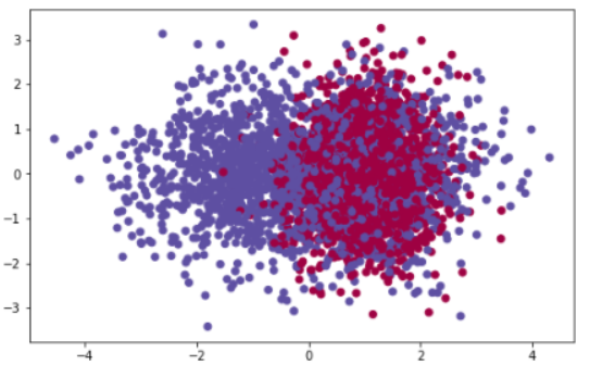
A plot of the data we want to classify
For this example, we will be using the bayes algorithm. To do this, our algorithm key is set to "bayes" in the configuration dictionary as follows:
# defining the configuration dictionary
config_dict = {"algorithm": "bayes",
               "spec": spec,
               "parameters": model_params,
               "name": "Bayes Optimization",
               "trials": 1}
The spec defines the specifications of the bayes algorithm. We are going to test 20 different combinations to see which combination can minimize the loss of our model.
# setting the spec for bayes algorithm
spec = {"maxCombo": 20,
        "objective": "minimize",
        "metric": "loss",
        "minSampleSize": 500,
        "retryLimit": 20,
        "retryAssignLimit": 0}
To train our model, we will be using a Random Forest classifier. There are several hyperparameters that we could tune, but for this example, we will only be tuning the number of estimators used to build the forest, the criterion to measure the quality of the split and the minimum number of samples required to be at a leaf node.
# setting the parameters we are tuning
model_params = {"n_estimators": {
                      "type": "integer",
                      "scaling_type": "uniform",
                      "min": 100,
                      "max": 300},
                "criterion": {
                      "type": "categorical",
                      "values": ["gini", "entropy"]},
                "min_samples_leaf": {
                      "type": "discrete",
                      "values": [1, 3, 5, 7, 9]}
}
Next, we initialize the Optimizer. To access your Comet dashboard, you’ll need to provide an api_key, which can be accessed through your Comet profile and account settings. You then assign the config_dict variable to the config parameter. I’ve also provided a project_name and workspace so the experiments are saved to a project I created in my dashboard.
# initializing the comet ml optimizer
opt = comet_ml.Optimizer(api_key="yaUBuGWQQel4gQ5TaNCWbYXal",
                         config=config_dict,
                         project_name="testing-hyperparameter-approaches",
                         workspace="kurtispykes")
Note: Never share API keys. Comet allows you to set your API key as a config variable. You can learn more about using this method here.
To begin, we loop through the experiments with the get_experiments() method. For each experiment, we define a Random Forest instance and use the get_parameter() method to get the parameter for the experiment being run.
We then train the model and make predictions on the test set. To demonstrate more of Comet’s functionality, I’ve saved the random_state value, the accuracy of the model on the test data, and a confusion matrix to get a better understanding of how the model performed.
Once the run is completed, we end the experiment and begin the next one until we’ve reached the maxCombo.
for experiment in opt.get_experiments():
    # initializing random forest
    # setting the parameters to be optimized with get_parameter
    random_forest=RandomForestClassifier(
        n_estimators=experiment.get_parameter("n_estimators"),
        criterion=experiment.get_parameter("criterion"),
        min_samples_leaf=experiment.get_parameter("min_samples_leaf"),
        random_state=25)

# training the model and making predictions
random_forest.fit(X_train, y_train)
y_hat = random_forest.predict(X_test)

# logging the random state and accuracy of each model
experiment.log_parameter("random_state", 25)
experiment.log_metric("accuracy", accuracy_score(y_test, y_hat))
experiment.log_confusion_matrix(y_test, y_hat)

experiment.end()
And that’s all.
We can view the experiments that were conducted from our dashboard:

experiment dashboard
By selecting an experiment, we can view different charts, code, hyperparameters, metrics, etc. This makes it easy to reproduce an experiment at any time in the future.
