Diffusion Language Models, From Scratch to Production

“Language model” used to be a very general term for statistical models trained to complete language tasks. It included everything from n-gram models to LSTMs and GRUs. But following the release of GPT-3.5 and ChatGPT, the term “language model” has had its definition—at least, from a general audience’s point of view—narrow considerably to specifically mean “autoregressive Transformers”. 

In 2026, however, we’ve started to see things broaden a bit. Different architectures have begun to move from the research realm into actual production settings. State-space models, so-called “looped Transformers”, and most prominently, diffusion models are suddenly genuine options for real-world use.

Much of the writing around these models frames the situation as “Is this generally superior to GPT-5.6?”, but this is the wrong way to evaluate them. Each new architecture brings with it particular tradeoffs that are useful in particular situations. The goal of this article is to shine a light on exactly what those tradeoffs are for diffusion language models.

What Actually Is A Diffusion Language Model?

Autoregressive language models generate text one token at a time, left to right. Once a token is generated, it’s fixed. Diffusion models take a different approach: they generate a whole sequence at once and refine it over multiple passes, so earlier tokens stay open to revision as the rest of the sequence takes shape.

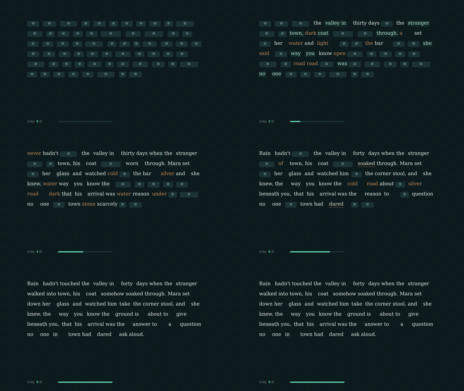
That difference (sequential generation versus parallel refinement) can sometimes make diffusion models faster, but also makes them fail differently. And it’s no longer a purely theoretical tradeoff. Google’s Gemini Diffusion remains competitive with autoregressive models on coding benchmarks while generating substantially faster, and its open successor, DiffusionGemma, runs up to 4x quicker than the autoregressive Gemma 4 it’s built from, though at some cost in quality. 

So the interesting question isn’t whether diffusion is simply “better” than autoregression. It’s when the speed is worth the quality tradeoff. 

We’ll answer that question in three steps:

1. Understand the math behind masked diffusion.
2. Build a tiny diffusion language model from scratch so we can see the mechanism directly.
3. Evaluate a production diffusion model with Opik to measure the quality/latency tradeoff rather than assuming it.

Why Diffusion For Text At All

Generating tokens sequentially carries a structural cost: once a token is emitted, it is never reconsidered. The model never revises an earlier word based on how the sentence turned out.

You’re probably familiar with diffusion models in the context of image generation. An image diffusion model takes a real image, adds Gaussian noise until it is pure static, and trains a network to reverse the process, recovering the image from noise one step at a time. Instead of committing in a single pass, it refines gradually and corrects itself along the way.

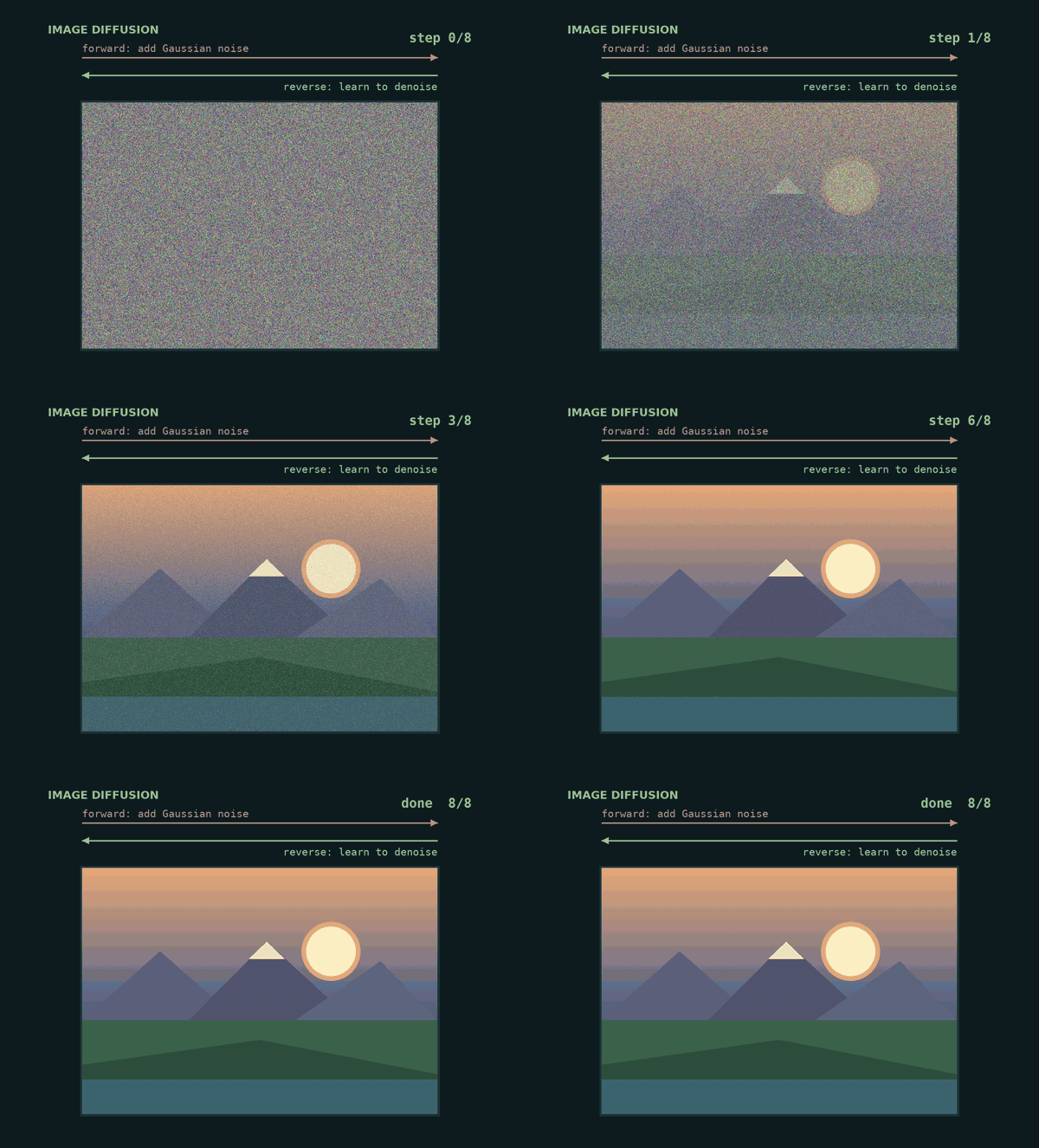
This process is commonly referred to as continuous diffusion, and it presents some challenges for language models. 

The fix is to redefine “adding noise” as masking. Replace some fraction of the tokens with a [MASK] symbol and train the model to recover them. At a 100% mask rate the sequence is blank; near 0% it is nearly intact, and the model learns to denoise at every level in between. As the next section shows, this is a generalization of BERT’s masked language modeling objective.

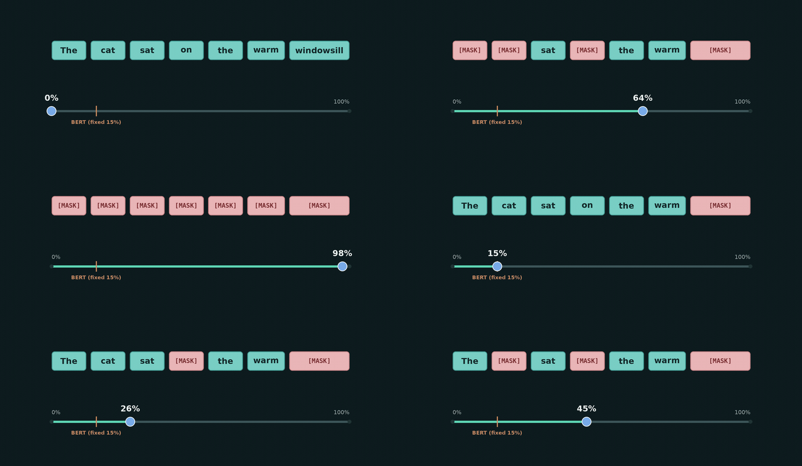
Masking gives diffusion two advantages.

The first is parallelism. Because the model predicts masked positions instead of extending a sequence, it can fill many positions at once. This is the speed argument, and the evaluation section below tests it directly.

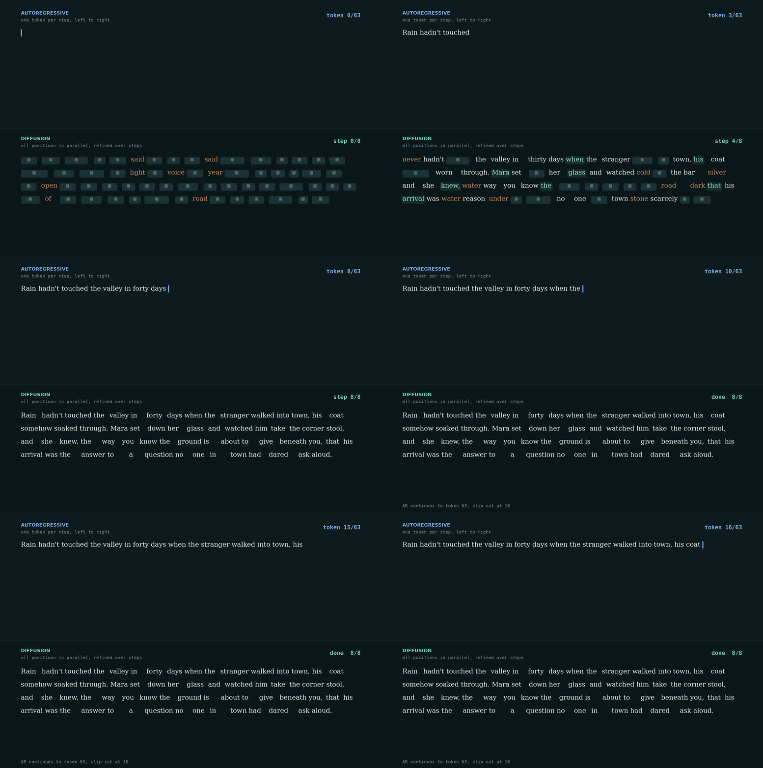
The second is bidirectional context. An autoregressive model attends only to tokens on its left, because the tokens on its right do not exist yet. A diffusion model sees the whole sequence at every step, so it can revise an earlier token as the later ones settle. DeepMind reports that this lets Gemini Diffusion correct errors during generation, which is why diffusion suits editing tasks in math and code. It also frees generation from left-to-right order, which makes infilling and constrained generation more natural, the motivation behind the original Diffusion-LM work (Li et al., 2022).

Both advantages are real in principle but show up unevenly in practice. Gemini Diffusion, for instance, matches its autoregressive counterpart on code while trailing it on multilingual and reasoning benchmarks, and parallelism shows why.

To decode in parallel, diffusion models assume the tokens produced in a single step are conditionally independent. In natural language they usually are not, and when the assumption breaks, quality drops. ParallelBench (Kang et al., 2025) shows this degradation is sharp on realistic tasks, and that current decoding strategies cannot adjust their parallelism to task difficulty, making speedup without a quality cost hard to reach. Which advantage wins depends on the task.

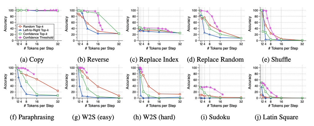
Underneath both advantages is a single idea: how much intermediary computation each one can do, the variable “work” a model puts in before committing to an answer. An autoregressive model does a fixed amount of work per token. When it needs to try harder, it does so by writing more tokens, which is what a long chain of reasoning is. A diffusion model works the other way, spending variable computation on a fixed set of tokens by refining them over more or fewer passes. One tries harder by writing more; the other tries harder by thinking longer about what it has already written.² If you have used a reasoning model’s effort settings, you have already met this tradeoff from the outside.

Knowing when to reach for diffusion means understanding how it works from the inside. That is where we start.

The Math

Masked diffusion comes down to three things: how you add noise, how the model removes it, and what it optimizes to learn that. Everything follows from those.

The forward process

Take a clean sequence of tokens, $x_0 = (x_0^1, \ldots, x_0^L)$.

The forward process corrupts it by masking. Pick a time t between 0 and 1. Under a linear schedule, each token is masked independently with probability t, replacing it with a special [MASK] symbol m.¹

For a single token, the probability of the corrupted value is:

$q(x_t^i \mid x_0^i) = (1 – t)\,\mathbf{1}[x_t^i = x_0^i] + t\,\mathbf{1}[x_t^i = m]$

In words: with probability 1−t the token is left alone, and with probability t it becomes [MASK]. So t is a dial for how corrupted the text is, fully intact at 0, fully masked at 1.

This is the discrete analogue of adding Gaussian noise to an image, where t plays the same role the noise level does for an image. The difference is that “noise” here is not a small perturbation of a value.It is the total erasure of a token, replaced by a single placeholder symbol.

The reverse process

Generation runs this backwards. The model is a denoiser: it takes a partially masked sequence x_t and predicts the original token at every masked position at once. Call i $p_\theta(x_0^i \mid x_t)$, the model’s distribution over what the true token was, for each masked position i.

Two properties matter here. The model conditions on the entire sequence x_t, both the masked positions and the unmasked ones on either side. It attends in both directions. And it predicts all masked positions in a single forward pass, which is where the parallelism comes from.

That second property is easy to misread. Predicting all masked positions at once does not mean predicting them independently of one another in the final output. A single denoising step does treat the masked positions as conditionally independent given x_t, the assumption that makes the parallel prediction tractable, but generation is not a single step. It runs many steps, and each step reveals a few tokens and feeds them back as context for the next. The dependencies between tokens are reintroduced across steps, through the model re-attending to what it has already committed. This is exactly the trade the ParallelBench work probes: commit too many tokens per step and you lean too hard on the independence assumption; commit too few and you lose the speed that made diffusion attractive.

The training objective

The model learns by trying to reverse the corruption. Sample a clean sequence, sample a time t, mask the sequence accordingly, and ask the model to predict the original tokens at the masked positions. Score it with cross-entropy, evaluated only where tokens were masked:

$\mathcal{L} = -\,\mathbb{E}_{t,\,x_0,\,x_t}\left[ w(t) \sum_{i=1}^{L} \mathbf{1}[x_t^i = m] \log p_\theta(x_0^i \mid x_t) \right]$

The indicator restricts the loss to masked positions; the model gets no credit for copying tokens it was handed. The weight w(t) rescales the loss by time step. With the weighting the objective derives to, the summed loss is a variational bound on the sequence log-likelihood, which is what lets you sample from the trained model as a generator rather than use it only for fill-in-the-blank prediction like BERT. In practice, implementations sometimes simplify or adjust this weighting for stability, trading a little theoretical tightness for easier training. This is the simplified form from the MDLM work (Sahoo et al., 2024), whose full derivation is worth reading there; the object you actually optimize is the weighted masked cross-entropy above.

If that objective looks familiar, it should. Masking tokens and predicting them from bidirectional context is BERT’s masked language modeling objective. The difference is that BERT masks at a single fixed rate, around 15%, while masked diffusion trains across every masking rate from 0 to 100%, sampled through t. Masked diffusion is masked language modeling extended over a continuum of corruption levels, which turns a representation-learning objective into a generative one. Train BERT to fill in blanks at every possible density of blanks, and you can generate by starting from all blanks and filling them in.

The next section builds exactly this: a bidirectional encoder trained with masked cross-entropy, sampled by starting from a fully masked sequence and denoising it step by step.

Building a Diffusion LM From Scratch

The model here is deliberately tiny: character-level, trained on a handful of sentences, small enough to run in a notebook on CPU in a couple of minutes. It will only ever reassemble the few sentences it was trained on, but that is enough to see the mechanism work. The masking, the bidirectional denoiser, and the step-by-step sampling from the previous section all become concrete in the code below. You can run it and see for yourself how the step count changes the output.

Follow along with the Colab: https://colab.research.google.com/drive/1UgA3udHN0dznuGTkmeCLzZCZjjkyhc7e

Data and vocabulary

Start with a small corpus of simple sentences and a character-level vocabulary. The only unusual piece is the mask token: it gets an id one past the real characters, so the model has a symbol that means “something was here.”

text = (
    "the cat sat on the mat. "
    "the dog ran in the park. "
    "a bird flew over the tree. "
    "the fish swam in the pond. "
    "the sun set behind the hill. "
) * 200

chars = sorted(set(text))
stoi = {c: i for i, c in enumerate(chars)}
itos = {i: c for c, i in stoi.items()}
MASK = len(chars)          # mask token id: one past the real vocab
VOCAB = len(chars) + 1     # real characters + [MASK]
BLOCK = 24

The forward process in code

This is the masking equation from the previous section, written directly. Sample a masking rate t per sequence, then mask each token independently with probability t. That comparison, torch.rand_like(x) < t, masks each position with probability t, which is the linear schedule from the math: the mask rate is just t itself.

def add_noise(x):
    # forward process: this is q(x_t | x_0) from the math, applied to a whole batch
    t = torch.rand(x.size(0), 1)                        # sample a masking rate t ~ U(0,1) per sequence
    mask = torch.rand_like(x, dtype=torch.float) < t    # mask each token independently with probability t
    xt = torch.where(mask, torch.full_like(x, MASK), x) # masked -> [MASK], else keep original
    return xt, mask, t.squeeze(1)                       # mask marks which positions the loss will score

The returned mask tells us which positions were corrupted, which is all the training loop needs to score the model only where it had to guess.

The denoiser

The model is a standard transformer encoder. There is one line that makes it a diffusion model rather than a language model in the usual sense, and it is a line you do not write: there is no causal mask. The encoder attends in both directions, so every position sees the whole sequence, exactly the bidirectional property from the math.

class Denoiser(nn.Module):
    def __init__(self, vocab=VOCAB, d=64, heads=4, layers=2, block=BLOCK):
        super().__init__()
        self.tok = nn.Embedding(vocab, d)
        self.pos = nn.Embedding(block, d)
        self.time = nn.Sequential(nn.Linear(1, d), nn.GELU(), nn.Linear(d, d))
        enc = nn.TransformerEncoderLayer(d, heads, dim_feedforward=4*d,
                                         batch_first=True,activation="gelu")
        self.blocks = nn.TransformerEncoder(enc, layers)
        self.ln = nn.LayerNorm(d)
        self.head = nn.Linear(d, vocab)

    def forward(self, x, t):
        pos = torch.arange(x.size(1))
        h = self.tok(x) + self.pos(pos)[None]      
        h = h + self.time(t[:, None])[:, None, :]   # condition on noise level: same t as the forward process
        h = self.blocks(h)                          # no causal mask: every position attends both directions
        return self.head(self.ln(h))                # logits over vocab at every position = p_theta(x_0 | x_t)

If you have built a GPT-style model before, this is that same architecture with the causal mask removed. That single change, letting every position see the whole sequence, is what makes it a diffusion denoiser instead of an autoregressive model.

The training loop

The training loop is simply the loss equation from the previous section, turned into code: corrupt a batch, predict the originals, and take cross-entropy on the masked positions only.

def train(steps=2500, lr=3e-4):
    model = Denoiser()
    opt = torch.optim.AdamW(model.parameters(), lr=lr)
    for step in range(steps):
        x = get_batch()
        xt, mask, t = add_noise(x)
        logits = model(xt, t)
        # cross-entropy only on masked positions: the indicator 1[x_t = MASK] from the loss equation
        loss = F.cross_entropy(logits[mask], x[mask])   # loss only where masked
        opt.zero_grad(); loss.backward(); opt.step()
    return model

The logits[mask] indexing does the job of the indicator in the loss equation: it selects only the masked positions, so the model is scored on what it had to guess and gets nothing for the tokens it was handed.” Running this drops the loss from about 3.3 to around 1.0 in a couple of minutes on CPU.

The sampling loop

This is the reverse process, and it is where the step-count knob lives. Start from a fully masked sequence and denoise it over n_steps iterations. At each step, the model predicts every masked position, and we commit only a fraction of them, (the ones the model is most confident about) feeding those back as context for the next step. Committing the most confident predictions first is what lets each step build on the tokens the previous steps got right.

@torch.no_grad()
def sample(model, n_steps, length=BLOCK):
    # reverse process: start fully masked, then unmask a few positions at a time over n_steps
    x = torch.full((1, length), MASK, dtype=torch.long) # x at t=1: everything masked
    reveal_per_step = math.ceil(length / n_steps)       # how many to commit each step
    for s in range(n_steps):
        t = torch.tensor([(x[0] == MASK).float().mean()])   # current noise level = fraction still masked
        probs = F.softmax(model(x, t), -1)[0]               # p_theta(x_0 | x_t) at every position
        pred = torch.multinomial(probs, 1).squeeze(-1)      # sample a token per position
        conf = probs.gather(-1, pred[:, None]).squeeze(-1)  # model's confidence in each sampled token

        masked = (x[0] == MASK)
        if masked.sum() == 0:
            break
        # remasking strategy: keep only the most confident predictions, leave the rest masked for next step
        cand = torch.where(masked, conf, torch.full_like(conf, -1.0))
        k = min(reveal_per_step, int(masked.sum().item()))
        idx = torch.topk(cand, k).indices
        x[0, idx] = pred[idx]                               # commit those tokens; they become context next step
    # fill any positions still masked after the last step
    left = (x[0] == MASK)
    if left.any():
        x[0, left] = model(x, torch.tensor([0.0]))[0, left].argmax(-1)
    return "".join(itos[i.item()] for i in x[0])

Two knobs control everything here: n_steps, the number of denoising iterations, and the rule for how many positions to reveal per step. Both trade quality against speed, and both are exactly what a production diffusion model exposes, just at a larger scale.

Turning the step-count knob

Here is what that produces, the same trained model sampled at 2, 8, and 24 steps:

[ 2 steps] 'he on the ohta troc ' 
[ 8 steps] '. the the sat on the mat' 
[24 steps] '. the dog ran in the par'

At 2 steps the model commits almost everything at once, leaning entirely on the conditional-independence assumption, and the result has the right letter and spacing statistics but no structure. At 8 steps whole words hold together and a sentence starts to form. At 24 steps, one step per token, it recovers a clean sentence from the training text, “the dog ran in the par…”, because each step commits only a few positions and lets the rest condition on them.

This is the core diffusion tradeoff, visible in miniature: more steps, better output, more compute. It is the same curve the evaluation section measures on production models, and here you can see exactly where it comes from. You can see the independence assumption from the math directly in the 2-step sample: commit that many tokens at once and it falls apart.

One thing this model does not do is generate novel text. It has five sentences of training data and a few dozen characters of vocabulary, so when it produces something clean, it is reassembling sentences it has seen, not composing new ones. That is the difference between a teaching artifact and a working model. The mechanism we built is exactly what a production diffusion model uses: masking, a bidirectional denoiser, and iterative unmasking.What a production model adds is scale: enough parameters and data to generalize instead of memorize. The next section evaluates models that have made that jump.

Evaluating production diffusion LLMs with Opik

The toy model showed the mechanism. It cannot tell you whether diffusion is worth using, because it only memorizes a handful of sentences and runs on a CPU. To find out, we evaluate a production diffusion model the way you would evaluate any model headed for production: run it on a fixed task, trace every call, and score the outputs on the things you actually care about.

An autoregressive model and a diffusion model are two ways to spend intermediary computation, and they spend it differently: an autoregressive model does more work by writing more tokens, while a diffusion model does more work per token. That difference tells us what to measure. Quality says whether the answer is right; latency and output tokens say what each model spent to get there and whether the two paradigms spend differently in practice.We compare one diffusion model, Inception’s Mercury 2, against a cost-matched autoregressive baseline, Claude Haiku 4.5, on a set of small code-generation tasks.

We use code generation because it’s verifiable: the output either passes a test or it doesn’t.

The setup

Follow along in the Colab here: https://colab.research.google.com/drive/1BGfRh4W-ULOTa-U659ZvY-cYTkPGzEc_ 

You can follow along in the companion notebook. It uses Opik’s hosted free tier by default, so it runs without any setup. If you’d rather self-host the open-source version, follow the instructions in the Opik repo and update the OPIK_URL variable at the top of the notebook to point at your local instance.

Both models are called through LiteLLM, which gives them the same interface, so the only thing that changes between runs is the model name. Opik handles the tracing. Wrapping the LiteLLM call with track_completion means every request is logged automatically, with its latency and token usage attached.

tracked_completion = track_completion()(litellm.completion)

def generate(prompt: str, model: str, **kwargs) -> dict:
    t0 = time.time()
    resp = tracked_completion(
        model=model,
        messages=[{"role": "user", "content": prompt}],
        **kwargs,
    )
    return {
        "text": resp.choices[0].message.content or "",
        "latency_s": time.time() - t0,
        "output_tokens": getattr(resp.usage, "completion_tokens", None),
    }

The tasks are graded into easy, medium, and hard tiers, so we can see how each model behaves as problems get harder. Each prompt pins the function name so the test knows what to call.

The evaluation metric

We run the model’s code against the task’s test, and score 0 for anything that raises an exception. Before running it, we strip the Markdown fences models wrap code in, since they aren’t valid Python, and because each prompt pins the function name, the test can always find the function to call.

class CodePasses(base_metric.BaseMetric):
    def __init__(self, name: str = "code_passes"):
        self.name = name

    def score(self, output: str, test: str, **kwargs):
        try:
            scope = {}
            exec(extract_code(output), scope)
            exec(test, scope)
            passed = True
        except Exception:
            passed = False
        return score_result.ScoreResult(name=self.name,
                                        value=1.0 if passed else 0.0)

The evaluation task itself returns only what the metric scores. The other measurements, latency, output tokens, and difficulty, are logged to the Opik trace, where they can be compared and filtered without interfering with scoring.

def eval_task(item, model, **gen_kwargs):
    r = generate(item["prompt"], model, **gen_kwargs)
    opik_context.update_current_trace(
        metadata={"difficulty": item["difficulty"]},
        feedback_scores=[
            {"name": "latency_s", "value": float(r["latency_s"])},
            {"name": "output_tokens", "value": float(r["output_tokens"] or 0)},
        ],
    )
    return {"output": r["text"], "test": item["test"]}

For open-ended or non-verifiable tasks, we could swap our pass/fail metric for one of Opik’s built in LLM-as-a-judge metrics and run them alongside the latency and output_tokens logged as feedback scores above.

Comparing diffusion and autoregressive LMs

Running the evaluation over all thirty tasks, averaged across twenty runs, gives a clearer picture than a single pass would. Overall, Mercury 2 answered about twice as fast as Haiku (3.0s versus 6.0s on average) while passing fewer tasks (84% versus 99.7%). But the overall number hides the more interesting result, which only shows up when you break performance down by difficulty.

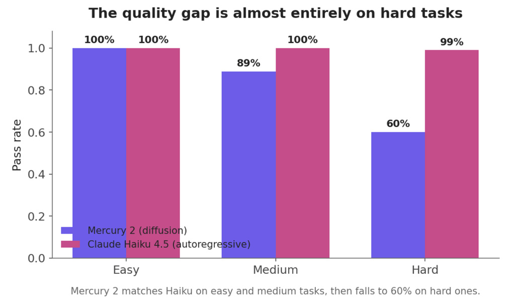
The quality gap is almost entirely on hard tasks. On easy problems the two models are identical, both at 100%. On medium ones Mercury slips slightly, 89% to Haiku’s 100%. It is only on the hard tier that they diverge sharply: Mercury passes 60% where Haiku passes 99%. So this isn’t a model that’s uniformly a bit worse. It’s a model that matches a strong autoregressive baseline until the problem gets genuinely hard, then falls off.

The speed advantage, meanwhile, holds at every level, and widens with difficulty.

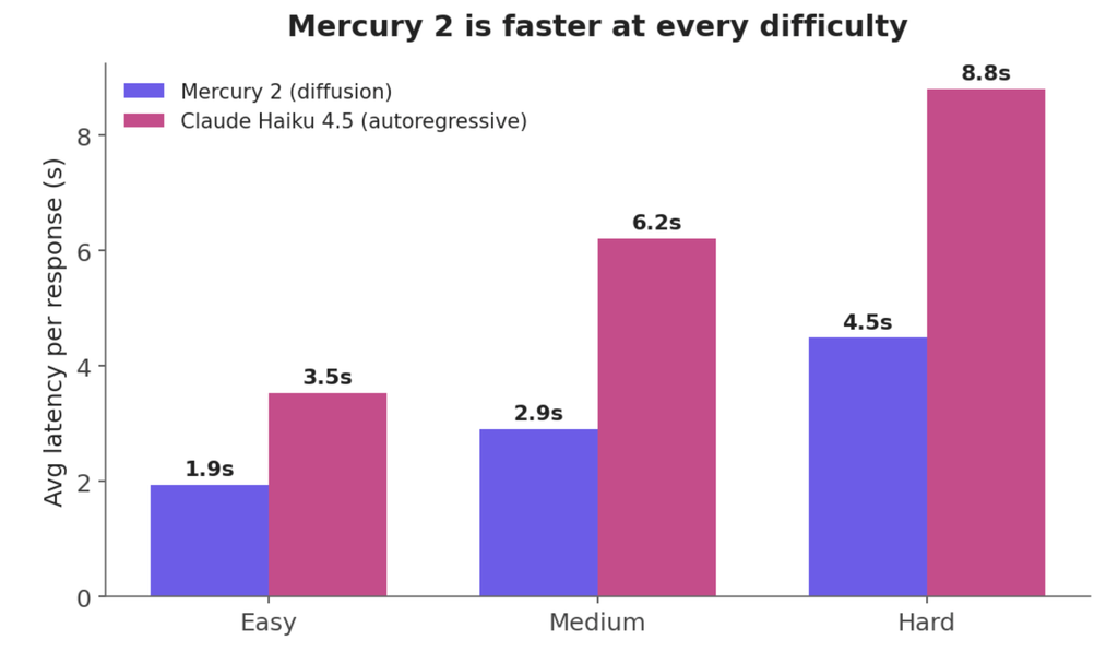
Mercury was faster on every tier, and the gap grew as tasks got harder: roughly 1.9s versus 3.5s on easy tasks, but 4.5s versus 8.8s on hard ones. Both models spent more time and more tokens on harder problems, and interestingly, they spent them similarly, output token counts were nearly identical between the two (689 versus 714 on average). The difference wasn’t in how much either model wrote; it was that Haiku’s extra work on hard tasks cost roughly twice the wall-clock time.

Which model you’d choose comes down to where your tasks fall. For work that stays in easy-to-medium territory, Mercury gives you the same quality at half the latency, a clear win. For work heavy in genuinely hard problems, Haiku’s near-perfect accuracy is worth its slower responses, unless a wrong answer is cheap to catch, in which case Mercury’s speed may still be the better trade.

Turning the effort dial

Mercury 2 exposes a reasoning_effort setting, its control for how much computation to spend per response, from instant up to high. The question the toy model raised was whether spending more computation produces better answers. Sweeping all four levels across the same thirty tasks answers it, and the answer is more nuanced than a simple yes or no.

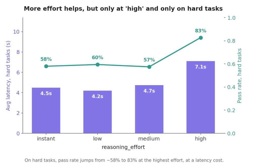
For most of the range, turning the dial up does very little. Across instant, low, and medium, hard-task pass rate barely moves, hovering around 58%, while latency drifts up only slightly. Then at high, something changes: pass rate on hard tasks jumps to 83%, a 25-point gain, and latency climbs with it, from roughly 4.5s to 7.1s.

Two things are worth drawing out. First, the extra computation does convert into better answers, but only at the top of the range and only where the problem is hard enough to use it. On easy and medium tasks, higher effort barely changed the outcome, those problems were already solved at low effort, so more computation was just more latency. The gains concentrated exactly where the model was struggling. Second, the payoff is discontinuous: three of the four settings behave almost identically, and all the improvement is packed into the jump to high.

This is the intermediary-computation idea made concrete. Mercury’s lever for spending more work is real, and when a hard problem demands it, pushing that lever to its limit recovers a large share of the accuracy the model otherwise loses. It just doesn’t do much until you push it all the way, and on easy work there’s nothing to recover, so the spend is wasted.

Reading the results honestly

The latency figures are end-to-end API times, which include network and provider-side serving, not just each model’s own compute, so they reflect what you’d experience as a user rather than a clean measurement of the paradigm. And reasoning_effort is a black box: Inception doesn’t document what it changes internally, so we can measure what it costs and returns, but not what it does under the hood.

None of this is settled, and the tradeoff isn’t specific to this one comparison. A June 2026 analysis benchmarked eight diffusion LLMs and showed that quality and cost trade off differently depending on denoising steps, block size, and how aggressively you unmask in parallel: more compute helped coding up to a point, saturated on math, and actively hurt translation. Block size cuts the same way, with small blocks refining well but decoding slowly and large blocks parallelizing at the cost of premature commitments. The point of instrumenting these runs is not to crown a winner but to see where on that surface your workload lands.

When Diffusion LMs Make Sense

Whether diffusion wins depends on the task, and our evaluation shows the shape of it, though what it directly establishes is narrow. On code-generation tasks, Mercury 2 matched a strong autoregressive baseline on easy and medium problems while halving latency, then fell behind on the hardest ones, where more computation helped only at the highest effort setting.

The dial Inception exposes is one instance of a larger pattern. A recent interpretability paper compared decoding orders on Dream-7B and found that decoding random positions first scored 8% on GSM8K while decoding the most confident positions first scored 56 to 59%, a far wider swing than any setting on a production API will show you. How you run a diffusion model matters as much as which one you pick.

From there, the mechanism suggests where the pattern should generalize. Diffusion’s advantage is parallelism, so it should pay off where latency is the binding constraint and the output is short enough to resolve in a few passes: code completion, on-device inference, high-throughput serving. The weakness is the mirror image, long, dependent generation, where the conditional-independence assumption behind parallel decoding breaks down and an autoregressive model’s left-to-right commitment becomes a feature rather than a limitation. Streaming is awkward for a related reason: a diffusion model refines the whole sequence at once, so there’s no natural way to emit it token by token. These claims extend past what we measured, but they follow from the same tradeoff the evaluation made concrete.

Diffusion is not a replacement for autoregressive generation, and the people building it are not claiming it is. Google’s own guidance for DiffusionGemma says as much: autoregressive for maximum quality, diffusion for speed-critical work. Our evaluation reached the same conclusion from the other direction. Diffusion is a different way to spend computation, faster when the work parallelizes, weaker when it doesn’t, and worth understanding because that tradeoff is becoming one you can choose.

Footnotes

¹“Writing more tokens” here means the reasoning tokens a model generates to work through a problem, not the explanation it may produce afterward to justify its answer. The former is computation toward the answer; the latter may be at least partly presentation rather than additional reasoning. There’s an active line of work suggesting the gap can be wider still, that even a model’s stated reasoning is not always a faithful account of its internal computation (Barez et al., 2025; Zaman et al., 2025 ; Arcuschin et al., 2025, Chen et al., 2025).

 ²Under the linear schedule the masking probability equals t directly, which keeps the notation clean. More generally the probability is 1−α_t​ for a monotonically decreasing schedule α_t​, and the loss weight w(t) depends on that choice. The linear case is enough to build and understand the model; see Sahoo et al. (2024) for the general treatment.