
Decision models drew wide attention in September, when TypeSafe AI launched Jev, a model that returns probabilities over a fixed set of answers instead of generating text. Open-source alternatives followed almost immediately: Latent.Space counted six in two days.
Most writing about decision models since then defines them by their interface, which uses some sort of schema or structured output. But an LLM with structured output produces something almost identical. What makes decision models unique is how they generate this output and what their probabilities are trained to mean.
This article explains that difference and what it changes in practice. It defines what a decision model is, builds a small one on a transformer backbone, tracks its training in Comet, and tests the trained model in Opik to check whether it has the properties that decision models promise.
What is a decision model?
A decision model takes an input, along with one or more questions whose possible answers are declared in advance, and returns a probability for each answer. The clearest way to see what that changes is to compare it with how an LLM produces structured output.
A structured-output LLM generates an answer token by token and constrains those tokens to fit the provided schema. Each output token costs another forward pass, later answers in the same response are conditioned on earlier ones, and the only probabilities available describe the next token rather than whether the answer is right.
By contrast, a decision model reads a probability for every allowed answer from a single pass, and those probabilities are trained to match how often each answer turns out to be right. This means cost and latency depend on the input rather than the length of the answer, several questions about the same input can be answered without influencing each other, and a 0.9 is meant to be right about 90% of the time.
Decision models vs. classifiers
If that sounds like a classifier, it’s because a decision model is much closer to one than to a chatbot. Transformer models come in two broad families. BERT-style encoders read the whole input at once, with every token able to attend to every other token in both directions, and they’re pretrained by predicting hidden words from the context on either side. With a small head on top, they’ve been the standard tool for classifying sentiment, spam, or intent since BERT came out in 2018. GPT-style decoders read left to right and are trained to predict the next token. They’re built to generate.
A decision model does the encoder’s job: read the input and return a distribution over answers. What’s changed is where the task comes from. A classic BERT classifier fixes its labels at training time, so adding a label means retraining the head. A decision model receives its questions and options with each request. A common summary of Jev is that it’s BERT-like, but with the data, compute, and training recipe of modern LLMs. TypeSafe hasn’t published Jev’s backbone, so that describes the approach rather than a confirmed architecture.
Calibration
The difference in what the probabilities mean comes from training. LLMs are post-trained toward answers people prefer (RLHF) or answers that pass an automatic check (RLVR), and neither directly rewards a model for saying how likely it is to be right. TypeSafe trains Jev, for example, with a method it calls Reinforcement Learning for Calibrated Decisions (RLCD). The goal is calibration, or probabilities that match how often each answer turns out to be right.
Calibration is important because not every wrong decision costs the same. Missing an urgent ticket might cost far more than escalating one that could have waited, so the right cutoff isn’t always 0.5; it depends on what each mistake costs. Calibrated probabilities let you set that cutoff in code: escalate a ticket above 0.2, auto-approve a refund above 0.95, and send the uncertain cases to a person. The same model can serve all of those decisions, and when costs change, you move the threshold instead of retraining.
But ‘calibrated’ isn’t the same as ‘accurate.’ A model that says 0.6 on every item and is right 60% of the time is perfectly calibrated, but it tells you nothing about which items to trust.
Accuracy measures how often the top answer is right. Calibration measures whether the probabilities match how often answers turn out right, so a model can be accurate and overconfident, or calibrated and barely better than guessing, and a useful decision model needs both.
When to use a decision model
Decision models don’t replace LLMs. LLMs remain the right tool for open-ended work like chat, coding agents, and anything that produces text a person reads. Decision models fit tasks where the possible answers can be listed in advance: classifying, routing, scoring, gating, and judging other models’ outputs, often at high volume or under tight latency limits.
| Generative LLMs | Decision models | |
| Returns | Text | A probability for each allowed answer |
| Answer space | Open. Output must be parsed and validated unless a schema constrains it. | Declared in advance; output is always one of the declared answers |
| How the output is produced | One token at a time, each conditioned on the ones before | Read out in a single pass |
| What the probabilities mean | Likelihood of the next token | Trained to match how often each answer turns out right |
| Cost and latency | Grow with input and output length | Grow with input length only |
| Several questions on one input | Later answers are conditioned on earlier ones | Can share one pass over the input while keeping questions independent |
| Explains its answer | Yes, it can write out its reasoning | No, it returns only the probabilities |
| Best fit | Open-ended work: chat, writing, code, agents | Tasks with answers you can list in advance: classifying, routing, scoring, gating, judging |
Build a small decision model
The clearest way to understand what makes a decision model unique is to build one. In this section, we’ll use Qwen3-0.6B-Base with LoRA adapters and a decision head trained from scratch on typed-decisions, a public benchmark on Hugging Face (Apache-2.0). Each case pairs one input, which Jev calls the state (for example, a summary of an agent’s run), with five typed questions about it. Every gold answer is a probability distribution rather than a single label.
We’ll break this down into four pieces: the data format, packing one state and several questions into a single sequence, the head that turns hidden states into probabilities, and the loss that trains those probabilities to mean something. The full code, including training, evaluation, and Comet logging, is in the companion repo. The excerpts below are trimmed, and some variable names are changed for readability.
The data
The typed-decisions benchmark covers four workflows:
- whether an agent run needs human review and how urgently
- the right response and action for a customer support thread
- whether to pay, hold, or reject a vendor invoice
- whether to close, investigate, or contain a security alert
Each case gives the model one state and asks five questions about it, mixing all three question types. In the agent-trace workflow, for example:
- choice: one of several named options (action, outcome)
- score: a level on an ordered scale (risk, urgency)
- noul: yes/no (needs_review)
A teacher model labeled each case three times, and the gold answer is the average of the three, so it stays spread out where a decision is ambiguous. In the case below, the teacher mostly wants a human review but puts some weight on stopping the agent. Training on these distributions teaches the model that an ambiguous case deserves an ambiguous answer.
Here’s one case from the agent-trace workflow, trimmed to three of its five questions, one of each type.
{
  "state": {"agent": {"autonomy": "unsupervised", "model": "internal-agent-v1"},
            "constraints": ["Never modify production without an approved change ticket"],
            "task": "Reconcile the billing ledger against the payment provider.",
            "trace_summary": {"constraint_violations": 1, "irreversible_actions": 1, "steps": 11, "tool_errors": 1}},
  "questions": {
    "action": {"type": "choice", "instructions": "What should the observability system do with this trace?",
               "criteria": {"continue": "Let the agent proceed without interruption.",
                            "human_review": "Queue this trace for a human to review.",
                            "observe": "Keep running, but flag the trace for later sampling.",
                            "stop": "Halt the agent now."}},
    "needs_review": {"type": "noul", "instructions": "This trace requires human review.",
                     "criteria": {"true": "A human should inspect this run.",
                                  "false": "No human attention is warranted."}},
    "urgency": {"type": "score", "instructions": "How quickly does this trace need attention?",
                "criteria": ["No time pressure; can wait indefinitely.",
                             "Routine; handle within the normal queue.",
                             "Elevated; should be handled within the same week.",
                             "Critical; requires action within the same day."]}
  },
  "gold": {
    "action": {"label": "human_review", "probabilities": {"continue": 0.02, "human_review": 0.70, "observe": 0.10, "stop": 0.18}},
    "needs_review": {"label": "true", "probabilities": {"false": 0.10, "true": 0.90}},
    "urgency": {"label": 3, "probabilities": {"0": 0.00, "1": 0.10, "2": 0.32, "3": 0.58}}
  }
}
Packing several questions in one pass
The two key advantages of decision models (that cost depends on the input rather than the answer, and that several questions about the same input can be answered without influencing each other) are both entirely dependent on how the input is laid out.
The straightforward way to ask five questions about one state is to run five separate sequences, each repeating the state. That works, but the model reads the same state five times. Instead, we put the state and all five questions into a single sequence:
[state][question 1 ... Answer:][question 2 ... Answer:] ... [question 5 ... Answer:]On a T4, packing five questions cut the tokens processed by 2.1 times and the time per case from 329 to 175 ms.
The attention mask: questions see the state, not each other
Packing creates a problem, though. A transformer normally lets every token look back at every token before it, so question 3 could read questions 1 and 2, and its answer could change depending on what else was asked. An attention mask controls which tokens each token is allowed to look at. In our case this means every question can see the state, and no question can see another question.
To build the attention mask, each token is tagged with the part of the sequence it belongs to: 0 for the state, 1 for the first question, and so on. A token can look back at an earlier token only if that token belongs to the state or to the same question:
def build_attention_mask(segment_ids: list[int]) -> torch.Tensor:
    seg = torch.tensor(segment_ids)
    causal = torch.ones(len(seg), len(seg), dtype=torch.bool).tril()
    same_question = seg[:, None] == seg[None, :]
    is_state = (seg == 0)[None, :]
    return causal & (same_question | is_state)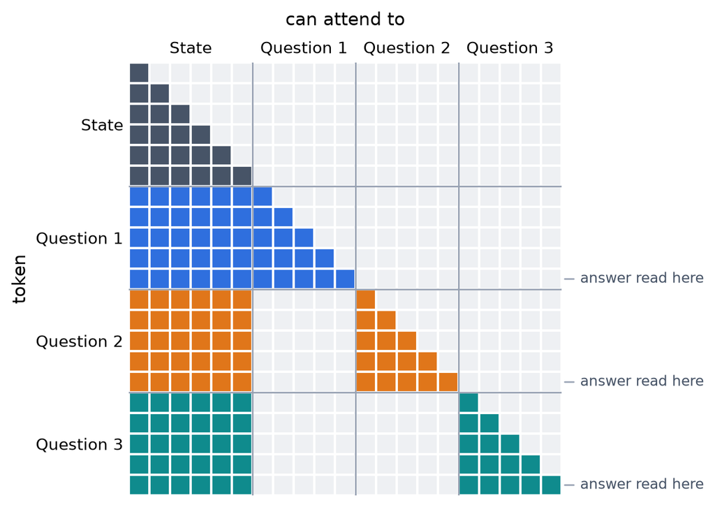
Positions: each question starts where the state ends
There’s one more detail worth noting. A transformer also tracks each token’s position, and a question placed fifth in the sequence would see different positions than it would if asked alone. So each question’s positions restart right after the state:
for i, question in enumerate(example.questions, start=1):
    tokens = tokenizer.encode(format_question(question), add_special_tokens=False)
    input_ids += tokens
    position_ids += range(state_len, state_len + len(tokens))  # restart after the state
    segment_ids += [i] * len(tokens)
    decide_index.append(len(input_ids) - 1)  # where the answer is read
With the mask and the restarted positions, the model treats each question as if it had been asked on its own: question 3 gets the same answer whether it’s packed with the other four or it’s run alone after the state. The repo’s tests check this to within floating-point error. In this way, packing changes the cost without affecting the answers. The state is processed once, however many questions you ask.
The decision head: from hidden state to probabilities
After packing, each question’s last token has only seen the full state and its own question, which are summarized in its hidden state. A regular LLM would pass this vector to its language-model head, which gives a probability for every possible next token. We pass it to a decision head instead, which gives a probability for each of the question’s allowed answers.
For choice and score questions, a linear layer maps the hidden state to one score (a logit) per option, and softmax turns the scores into probabilities. Slot 1 is the first option listed, slot 2 the second, and so on. Score questions work the same way, with one slot per level, in order.
A linear layer has a fixed number of outputs, but questions have different numbers of options, so the head is sized for the largest question it supports (16 options in the repo). For a question with fewer options, the extra outputs are masked out before the softmax and get zero probability.
Yes/no questions need only one number, z. The head returns the pair [0, z], and softmax over that pair gives P(yes) = sigmoid(z). Expressing yes/no this way means all three question types produce the same kind of output, so one loss and one set of metrics cover all of them.
def forward(self, hidden, question_type, num_options):
    z = self.noul(hidden)  # yes/no: a single logit
    noul = torch.cat([torch.zeros_like(z), z, torch.zeros(len(z), self.max_options - 2)], dim=1)

    qtype = question_type[:, None]
    logits = torch.where(qtype == CHOICE, self.choice(hidden),
                         torch.where(qtype == SCORE, self.score(hidden), noul))

    slots = torch.arange(self.max_options)
    return logits.masked_fill(slots[None, :] >= num_options[:, None], float("-inf"))
Because slots are defined by position, the options themselves only arrive as text in the input, so the same head can answer questions whose options it has never seen. But this also opens a shortcut. If “billing” is always listed first, the head can learn that slot 1 means billing without reading the options at all. So training shuffles the order of choice options every epoch, and the only way to know which slot is which is to read the list. Score levels stay in order, since their order carries meaning.
Lastly, the head’s weights start at zero, so before any training every question gets a uniform distribution.
The loss: training the probabilities to mean something
Training adjusts the model’s weights to make the loss smaller, so its probabilities mean whatever the loss rewards. If the loss only rewarded ranking the right answer first, a 0.9 would just mean “my top pick.” We use cross-entropy against the gold distribution instead, which penalizes the model for putting low probability on answers the gold considers likely:
def decision_loss(logits, targets, batch_size):
    log_probs = logits.log_softmax(dim=-1)
    log_probs = log_probs.masked_fill(targets == 0, 0.0)  # unused slots are -inf, and 0 * -inf is undefined
    return -(targets * log_probs).sum() / batch_size
Cross-entropy is what statisticians refer to as a proper scoring rule, meaning its average loss is lowest when the prediction matches the true distribution. For needs_review, where the gold puts 0.9 on yes, predicting 0.9 gives a loss of 0.33, while an overconfident 0.99 gives 0.47 and a hedging 0.7 gives 0.44. The model does best by reporting exactly the confidence the data supports.
The baseline: reading answers from the language-model head
To see what the head and the loss contribute, we compare against reading answers from the LLM’s own next-token probabilities, as many open-source alternatives do. The baseline uses the same backbone, adapters, and packed input, but at each question’s last token it applies softmax over the language-model head’s scores for the answer tokens (“ A”, “ B”, and so on, or “ No” and “ Yes”). Each model below changes one thing from the row above it:
| Model | Trained on | Accuracy | KL | Brier | ECE |
| Prior (reads nothing) | n/a | 0.502 | 0.402 | 0.199 | 0.074 |
| Zero-shot baseline | nothing | 0.430 | 0.628 | 0.354 | 0.245 |
| Fine-tuned baseline (the usual recipe) | the gold label, scored against the full vocabulary | 0.714 | 0.290 | 0.119 | 0.134 |
| Baseline with our loss | the gold distribution, scored over the answer tokens | 0.768 | 0.110 | 0.059 | 0.011 |
| Decision model (decision head) | the gold distribution | 0.757 | 0.111 | 0.061 | 0.019 |
ECE compares each prediction’s confidence with the chance that a sample from the teacher agrees with its top answer.
Untrained, the baseline is worse than predicting each question’s label frequencies without reading the input. Fine-tuning fixes most of that. Changing the objective does the rest: scoring the gold distribution over the answer tokens, rather than the gold label against the full vocabulary, adds five points of accuracy, cuts KL by 62%, and halves Brier. It also makes the probabilities mean what they say. The models trained on our loss are calibrated to within one to two points straight out of training, while the fine-tuned baseline is overconfident by 13. Temperature scaling brings the baseline down to three, which is still worse than our models before any scaling.
Swapping the language-model head for a decision head changes nothing we can measure: every difference between the last two rows falls inside its 95% interval. With the same objective and the same packed input, the readout isn’t what separates them; the loss is.
Tracking in Comet
We make every decision on a validation set, 15% of each workflow’s training cases, and score the test set once at the end. Training updates the head and the LoRA adapters, and keeps the epoch with the lowest validation log loss. Each run is one command and one Comet experiment, which logs validation metrics by epoch, question type, and question, along with reliability diagrams, the data split, and the checkpoint:
python -m decision_model.train configs/decision_head.yamlAll of the runs in this article are in a public Comet project.
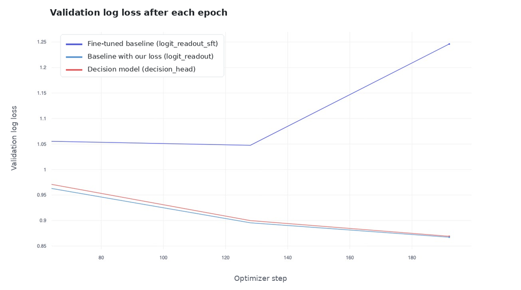
The two objectives diverge as training continues. The fine-tuned baseline’s validation log loss barely improves after its first epoch and rises sharply in its third, consistent with its probabilities growing more confident than its answers justify. The results use each model’s best epoch, so the baseline is judged at its second, before that rise, and it still trails. The two models trained on our loss improve through all three epochs and finish within 0.002 of each other.
The model is only as calibrated as its training labels, so the last step fits a temperature for each question type on validation data. It rescales confidence without changing the top answer, so calibration can improve while accuracy stays the same.
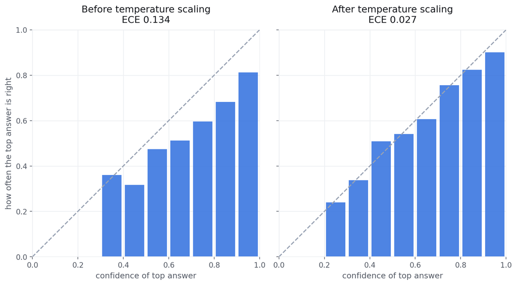
Before scaling, the fine-tuned baseline is overconfident at every confidence above 0.4: answers it gives more than 90% confidence agree with a teacher sample only about 81% of the time. Dividing its logits by about two moves the bars onto the diagonal and cuts ECE from 0.134 to 0.027. The models trained on our loss need almost no correction; their fitted temperatures are within 8% of 1.
Evaluating in Opik
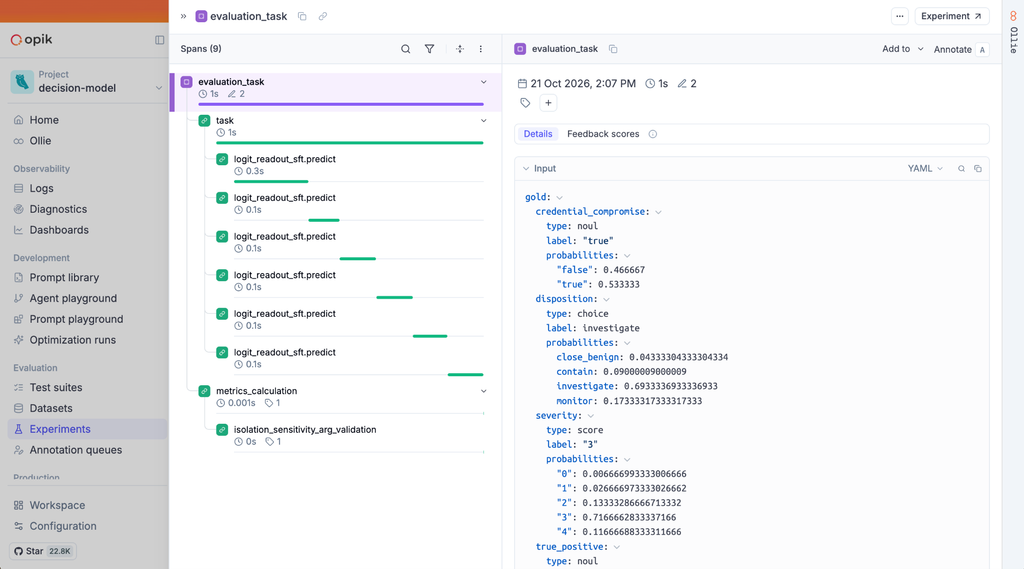
We made every modeling decision on validation, so the test set is scored only once, at the end, in Opik. Each of the 400 test cases becomes an Opik dataset item holding the request (the state and its questions) and the gold answers. Each model then runs as one experiment over all 400 cases.
Every model is called through the same function, predict(state, questions), which takes and returns the same request format as Jev. That means the same experiments could run against Jev, or any model that accepts that format.
python -m decision_model.opik_eval --runs outputs/logit_readout_sft outputs/logit_readout outputs/decision_head \
--zero-shot configs/logit_readout.yaml --split test| Model | Accuracy | KL | Brier | ECE |
| Zero-shot baseline | 0.43 | 0.63 | 0.35 | 0.25 |
| Fine-tuned baseline | 0.76 | 0.27 | 0.11 | 0.12 |
| Baseline with our loss | 0.78 | 0.10 | 0.05 | 0.02 |
| Decision model | 0.78 | 0.09 | 0.05 | 0.02 |
The test results match validation. The fine-tuned baseline’s accuracy gap is smaller on test, two points instead of five, but its calibration gap is the same: KL 0.27 against 0.10, and ECE 0.12 against 0.02. The decision head and the language-model head still score the same.
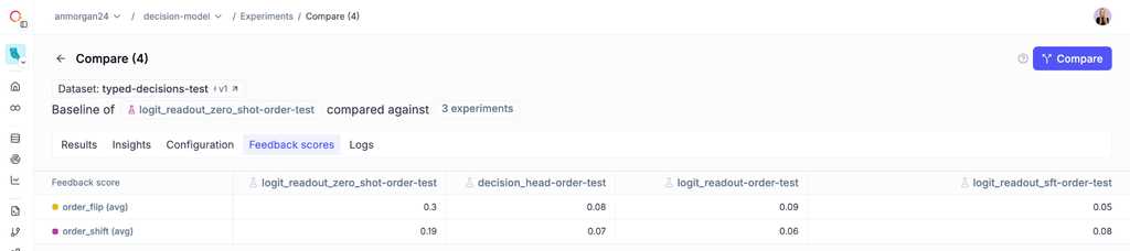
Accuracy and calibration don’t measure everything a decision model should do, so we ran three more experiments. Each one changes the request in a way that shouldn’t change the answer, then measures how much the answers move:
- Order: list each choice question’s options in reverse.
- Irrelevant option: add an option that has nothing to do with the decision.
- Isolation: ask each question on its own instead of all five together.
We measure each shift as the total variation distance between the two answer distributions, from 0 (identical) to 1 (no overlap).
| Model | Order: top answer changed | Order: shift | Irrelevant: probability taken | Irrelevant: shift | Isolation: shift |
| Zero-shot baseline | 30% | 0.19 | 3% | 0.04 | 0 |
| Fine-tuned baseline | 5% | 0.08 | 1% | 0.02 | 0 |
| Baseline with our loss | 9% | 0.06 | 4% | 0.03 | 0 |
| Decision model | 8% | 0.07 | 5% | 0.03 | 0 |
Option order has the largest effect. When the options are reversed, the untrained baseline changes its top answer on 30% of choice questions. In one customer-service case, the model is asked what the conversation is about. With the options listed alphabetically, it puts 0.96 on “technical.” With the options reversed, “technical” drops to 0.25 and “account” rises to 0.65. The trained models, which saw the options in shuffled order during training, change their answer on 5 to 9% of questions: far less, but not zero.
An irrelevant option has little effect on any model. It takes 1 to 5% of the probability and moves the other options by 2 to 4 points.
Isolation is 0 for every model, including the untrained one, because the attention mask makes it impossible for one question to affect another. For our models, the test confirms that the design works. It’s more useful for models whose internals you can’t inspect.
What this shows
A decision model is only useful if its probabilities mean what they say. In these experiments, that depended on how the model was trained, not on its architecture. Fine-tuned the standard way, on a single correct label per question, the model was overconfident (ECE 0.12 on the test set). Trained on the full gold distribution instead, its ECE was 0.02, with or without a dedicated decision head. Packing all five questions into one pass roughly halved the cost without changing any answer.
Training didn’t fix everything, though. When we listed the answer options in reverse order, the trained models still changed their top answer on 5 to 9% of questions.
The code, configs, and every run are public: the repo, the Comet project, and the Opik project.
