Author: Jeremy Jordan
Originally published at https://www.jeremyjordan.me on September 1, 2018, and was updated recently to reflect new resources.
The goal of this document is to provide a common framework for approaching machine learning projects that can be referenced by practitioners. If you build ML models, this post is for you. If you collaborate with people who build ML models, I hope that this guide provides you with a good perspective on the common project workflow. Knowledge of machine learning is assumed.
Overview
This overview intends to serve as a project “checklist” for machine learning practitioners. Subsequent sections will provide more detail.
Project lifecycle
Machine learning projects are highly iterative; as you progress through the ML lifecycle, you’ll find yourself iterating on a section until reaching a satisfactory level of performance, then proceeding forward to the next task (which may be circling back to an even earlier step). Moreover, a project isn’t complete after you ship the first version; you get feedback from real-world interactions and redefine the goals for the next iteration of deployment.
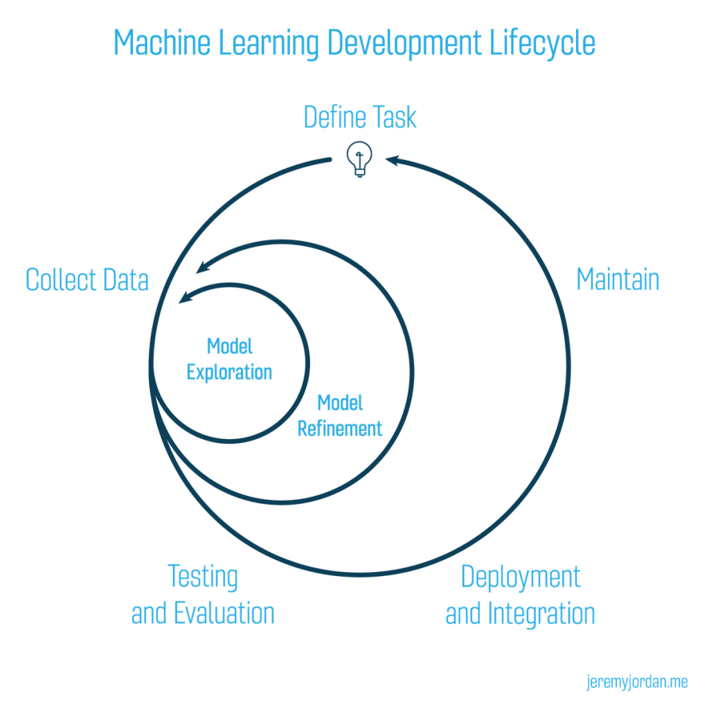
1. Planning and project setup
- Define the task and scope out requirements
- Determine project feasibility
- Discuss general model tradeoffs (accuracy vs speed)
- Set up project codebase
2. Data collection and labeling
- Define ground truth (create labeling documentation)
- Build data ingestion pipeline
- Validate quality of data
- Revisit Step 1 and ensure data is sufficient for the task
3. Model exploration
- Establish baselines for model performance
- Start with a simple model using initial data pipeline
- Overfit simple model to training data
- Stay nimble and try many parallel (isolated) ideas during early stages
- Find SoTA model for your problem domain (if available) and reproduce results, then apply to your dataset as a second baseline
- Revisit Step 1 and ensure feasibility
- Revisit Step 2 and ensure data quality is sufficient
4. Model refinement
- Perform model-specific optimizations (ie. hyperparameter tuning)
- Iteratively debug model as complexity is added
- Perform error analysis to uncover common failure modes
- Revisit Step 2 for targeted data collection of observed failures
5. Testing and evaluation
- Evaluate model on test distribution; understand differences between train and test set distributions (how is “data in the wild” different than what you trained on)
- Revisit model evaluation metric; ensure that this metric drives desirable downstream user behavior
- Write tests for: input data pipeline, model inference functionality, model inference performance on validation data, explicit scenarios expected in production (model is evaluated on a curated set of observations)
6. Model deployment
- Expose model via a REST API
- Deploy new model to small subset of users to ensure everything goes smoothly, then roll out to all users
- Maintain the ability to roll back model to previous versions
- Monitor live data and model prediction distributions
7. Ongoing model maintenance
- Understand that changes can affect the system in unexpected ways
- Periodically retrain model to prevent model staleness
- If there is a transfer in model ownership, educate the new team
Team roles
A typical team is composed of:
- data engineer (builds the data ingestion pipelines)
- machine learning engineer (train and iterate models to perform the task)
- software engineer (aids with integrating machine learning model with the rest of the product)
- project manager (main point of contact with the client)
Planning and project setup
It may be tempting to skip this section and dive right in to “just see what the models can do”. Don’t skip this section. All too often, you’ll end up wasting time by delaying discussions surrounding the project goals and model evaluation criteria. Everyone should be working toward a common goal from the start of the project.
It’s worth noting that defining the model task is not always straightforward. There’s often many different approaches you can take towards solving a problem and it’s not always immediately evident which is optimal. I’ll write a follow-up blog post with more detailed advice on developing the requirements for a machine learning project.
Prioritizing projects
Ideal: project has high impact and high feasibility.
Mental models for evaluating project impact:
- Look for places where cheap prediction drives large value
- Look for complicated rule-based software where we can learn rules instead of programming them
When evaluating projects, it can be useful to have a common language and understanding of the differences between traditional software and machine learning software. Andrej Karparthy’s Software 2.0 is recommended reading for this topic.
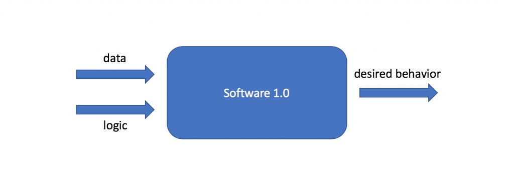
Software 1.0
- Explicit instructions for a computer written by a programmer using a programming language such as Python or C++. A human writes the logic such that when the system is provided with data it will output the desired behavior.
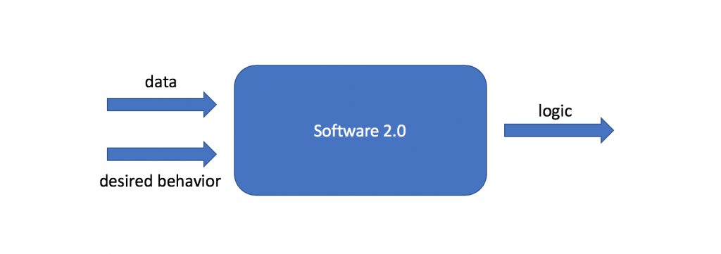
Software 2.0
- Implicit instructions by providing data, “written” by an optimization algorithm using parameters of a specified model architecture. The system logic is learned from a provided collection of data examples and their corresponding desired behavior.
See this talk for more detail.
A quick note on Software 1.0 and Software 2.0 — these two paradigms are not mutually exclusive. Software 2.0 is usually used to scale the logic component of traditional software systems by leveraging large amounts of data to enable more complex or nuanced decision logic.
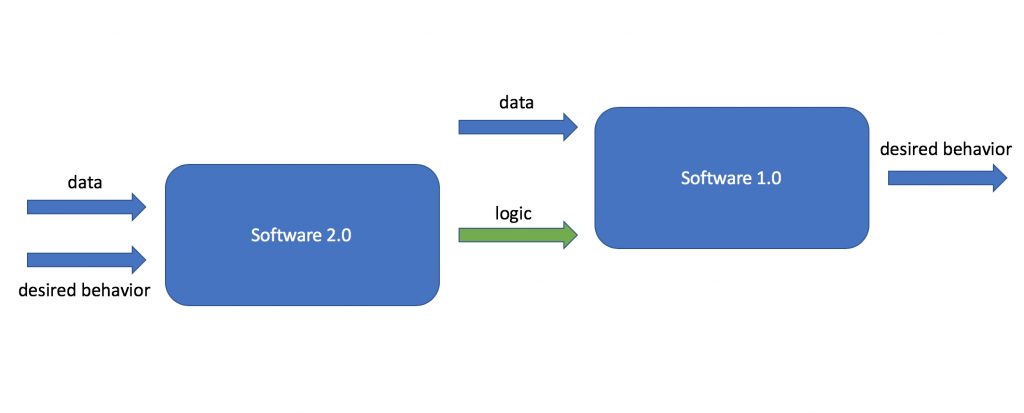
For example, Jeff Dean talks (at 27:15) about how the code for Google Translate used to be a very complicated system consisting of ~500k lines of code. Google was able to simplify this product by leveraging a machine learning model to perform the core logical task of translating text to a different language, requiring only ~500 lines of code to describe the model. However, this model still requires some “Software 1.0” code to process the user’s query, invoke the machine learning model, and return the desired information to the user.
In summary, machine learning can drive large value in applications where decision logic is difficult or complicated for humans to write, but relatively easy for machines to learn. On that note, we’ll continue to the next section to discuss how to evaluate whether a task is “relatively easy” for machines to learn.
Determining feasibility
Some useful questions to ask when determining the feasibility of a project:
- Cost of data acquisition
– How hard is it to acquire data?
– How expensive is data labeling?– How much data will be needed?
- Cost of wrong predictions
– How frequently does the system need to be right to be useful?
- Availability of good published work about similar problems
– Has the problem been reduced to practice?
– Is there sufficient literature on the problem?
- Computational resources available both for training and inference
– Will the model be deployed in a resource-constrained environment?
Specifying project requirements
Establish a single value optimization metric for the project. Can also include several other satisficing metrics (ie. performance thresholds) to evaluate models, but can only optimize a single metric.
Examples:
- Optimize for accuracy
- Prediction latency under 10 ms
- Model requires no more than 1gb of memory
- 90% coverage (model confidence exceeds required threshold to consider a prediction as valid)
The optimization metric may be a weighted sum of many things which we care about. Revisit this metric as performance improves.
Some teams may choose to ignore a certain requirement at the start of the project, with the goal of revising their solution (to meet the ignored requirements) after they have discovered a promising general approach.
Decide at what point you will ship your first model.
Some teams aim for a “neutral” first launch: a first launch that explicitly deprioritizes machine learning gains, to avoid getting distracted. — Google Rules of Machine Learning
The motivation behind this approach is that the first deployment should involve a simple model with focus spent on building the proper machine learning pipeline required for prediction. This allows you to deliver value quickly and avoid the trap of spending too much of your time trying to “squeeze the juice.”
Setting up a ML codebase
A well-organized machine learning codebase should modularize data processing, model definition, model training, and experiment management.
Example codebase organization:
|—— data/              <- raw and processed data for your project
|     |——README.md     <- describes the data for the project
|
|
|——docker/             <- specify one or many dockerfiles
|     |——dockerfile  <- Docker helps ensure consistent behavior
|                         across multiple machines/deployments
|
|
|——api/
|     |–—app.py        <- exposes model through REST client for
|                         predictions
|
|
|—— project_name/
|     |—— networks/    <- defines neural network architectures used
|     |     |——resnet.py
|     |     |—–densenet.py
|     |—— models/      <- handles everything else needed w/ network
|     |      |——base.py   including data preprocessing and output
|     |      |——simple_baseline.py                  normalization
|     |      |——cnn.py
|     |——configs/
|     |      |——baseline.yaml
|     |      |——latest.yaml
|     |——datasets.py   <- manages construction of the dataset
|     |——training.py   <- defines actual training loop for the model
|     |——experiment.py <- manages experiment process of evaluating
|                         multiple models/ideas. Constructs the
|                         dataset/model
|——scripts/
networks/ defines the neural network architectures used. Only the computational graph is defined, these objects are agnostic to the input and output shapes, model losses, and training methodology.
datasets.py manages construction of the dataset. Handles data pipelining/staging areas, shuffling, reading from disk.
experiment.py manages the experiment process of evaluating multiple models/ideas. This constructs the dataset and model for a given experiment.
training.py defines the actual training loop for the model, which is called by an Experiment object. This code interacts with the optimizer and handles logging during training.
Data collection and labeling
An ideal machine learning pipeline uses data which labels itself. For example, Tesla Autopilot has a model running that predicts when cars are about to cut into your lane. In order to acquire labeled data in a systematic manner, you can simply observe when a car changes from a neighboring lane into the Tesla’s lane and then rewind the video feed to label that a car is about to cut in to the lane.
As another example, suppose Facebook is building a model to predict user engagement when deciding how to order things on the newsfeed. After serving the user content based on a prediction, they can monitor engagement and turn this interaction into a labeled observation without any human effort. However, just be sure to think through this process and ensure that your “self-labeling” system won’t get stuck in a feedback loop with itself.
For many other cases, we must manually label data for the task we wish to automate. The quality of your data labels has a large effect on the upper bound of model performance.
Most data labeling projects require multiple people, which necessitates labeling documentation. Even if you’re the only person labeling the data, it makes sense to document your labeling criteria so that you maintain consistency.
One tricky case is where you decide to change your labeling methodology after already having labeled data. For example, in the Software 2.0 talk mentioned previously, Andrej Karparthy talks about data which has no clear and obvious ground truth.

If you run into this, tag “hard-to-label” examples in some manner such that you can easily find all similar examples should you decide to change your labeling methodology down the road. Additionally, you should version your dataset and associate a given model with a dataset version.
Tip: After labeling data and training an initial model, look at the observations with the largest error. These examples are often poorly labeled.
Active Learning
Useful when you have a large amount of unlabeled data, need to decide what data you should label. Labeling data can be expensive, so we’d like to limit the time spent on this task.
As a counterpoint, if you can afford to label your entire dataset, you probably should. Active learning adds another layer of complexity.
“The main hypothesis in active learning is that if a learning algorithm can choose the data it wants to learn from, it can perform better than traditional methods with substantially less data for training.” — DataCamp
General approach:
- Starting with an unlabeled dataset, build a “seed” dataset by acquiring labels for a small subset of instances
- Train initial model on the seed dataset
- Predict the labels of the remaining unlabeled observations
- Use the uncertainty of the model’s predictions to prioritize the labeling of remaining observations
Leveraging weak labels
However, tasking humans with generating ground truth labels is expensive. Often times you’ll have access to large swaths of unlabeled data and a limited labeling budget — how can you maximize the value from your data? In some cases, your data can have information which provides a noisy estimate of the ground truth. For example, if you’re categorizing Instagram photos, you might have access to the hashtags used in the caption of the image. Other times, you might have subject matter experts which can help you develop heuristics about the data.
Snorkel is an interesting project produced by the Stanford DAWN (Data Analytics for What’s Next) lab which formalizes an approach towards combining many noisy label estimates into a probabilistic ground truth. I’d encourage you to check it out and see if you might be able to leverage the approach for your problem.
Model exploration
Establish performance baselines on your problem. Baselines are useful for both establishing a lower bound of expected performance (simple model baseline) and establishing a target performance level (human baseline).
- Simple baselines include out-of-the-box scikit-learn models (i.e. logistic regression with default parameters) or even simple heuristics (always predict the majority class). Without these baselines, it’s impossible to evaluate the value of added model complexity.
- If your problem is well-studied, search the literature to approximate a baseline based on published results for very similar tasks/datasets.
- If possible, try to estimate human-level performance on the given task. Don’t naively assume that humans will perform the task perfectly, a lot of simple tasks are deceptively hard!
Start simple and gradually ramp up complexity. This typically involves using a simple model, but can also include starting with a simpler version of your task.
Once a model runs, overfit a single batch of data. Don’t use regularization yet, as we want to see if the unconstrained model has sufficient capacity to learn from the data.
- Practical Advice for Building Deep Neural Networks (see case study on overfitting an initial model)
Survey the literature. Search for papers on Arxiv describing model architectures for similar problems and speak with other practitioners to see which approaches have been most successful in practice. Determine a state of the art approach and use this as a baseline model (trained on your dataset).
Reproduce a known result. If you’re using a model which has been well-studied, ensure that your model’s performance on a commonly-used dataset matches what is reported in the literature.
Understand how model performance scales with more data. Plot the model performance as a function of increasing dataset size for the baseline models that you’ve explored. Observe how each model’s performance scales as you increase the amount of data used for training.
Model refinement
Once you have a general idea of successful model architectures and approaches for your problem, you should now spend much more focused effort on squeezing out performance gains from the model.
Build a scalable data pipeline. By this point, you’ve determined which types of data are necessary for your model and you can now focus on engineering a performant pipeline.
Apply the bias variance decomposition to determine next steps. Break down error into: irreducible error, avoidable bias (difference between train error and irreducible error), variance (difference between validation error and train error), and validation set overfitting (difference between test error and validation error).
If training on a (known) different distribution than what is available at test time, consider having two validation subsets: val-train and val-test. The difference between val-train error and val-test error is described by distribution shift.
Addressing underfitting:
- Increase model capacity
- Reduce regularization
- Error analysis
- Choose a more advanced architecture (closer to state of art)
- Tune hyperparameters
- Add features
Addressing overfitting:
- Add more training data
- Add regularization
- Add data augmentation
- Error analysis
- Tune hyperparameters
- Reduce model size
Addressing distribution shift:
- Perform error analysis to understand nature of distribution shift
- Synthesize data (by augmentation) to more closely match the test distribution
- Apply domain adaptation techniques
Use coarse-to-fine random searches for hyperparameters. Start with a wide hyperparameter space initially and iteratively hone in on the highest-performing region of the hyperparameter space.
- See Hyperparameter tuning for machine learning models.
Perform targeted collection of data to address current failure modes. Develop a systematic method for analyzing errors of your current model. Categorize these errors, if possible, and collect additional data to better cover these cases.
Debugging ML projects
Why is your model performing poorly?
- Implementation bugs
- Hyperparameter choices
- Data/model fit
- Dataset construction
Key mindset for DL troubleshooting: pessimism.
In order to complete machine learning projects efficiently, start simple and gradually increase complexity. Start with a solid foundation and build upon it in an incremental fashion.
Tip: Fix a random seed to ensure your model training is reproducible.
Common bugs:
Discovering failure modes
Use clustering to uncover failure modes and improve error analysis:
- Select all incorrect predictions.
- Run a clustering algorithm such as DBSCAN across selected observations.
- Manually explore the clusters to look for common attributes which make prediction difficult.
Categorize observations with incorrect predictions and determine what best action can be taken in the model refinement stage in order to improve performance on these cases.
Testing and evaluation
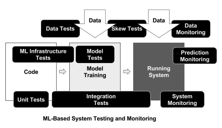
Different components of a ML product:
- Training system processes raw data, runs experiments, manages results, stores weights.
Required tests:
– Test the full training pipeline (from raw data to trained model) to ensure that changes haven’t been made upstream with respect to how data from our application is stored. These tests should be run nightly/weekly.
- Prediction system constructs the network, loads the stored weights, and makes predictions.
Required tests:
– Run inference on the validation data (already processed) and ensure model score does not degrade with new model/weights. This should be triggered every code push.
– You should also have a quick functionality test that runs on a few important examples so that you can quickly (<5 minutes) ensure that you haven’t broken functionality during development. These tests are used as a sanity check as you are writing new code.
– Also consider scenarios that your model might encounter, and develop tests to ensure new models still perform sufficiently. The “test case” is a scenario defined by the human and represented by a curated set of observations.
(Example: For a self driving car, you might have a test to ensure that the care doesn’t turn left at a yellow light. For this case, you may run your model on observations where the car is at a yellow light and ensure that the prediction doesn’t tell the car to proceed forward.)
- Serving system exposed to accept “real world” input and perform inference on production data. This system must be able to scale to demand.
Required monitoring:
– Alerts for downtime and errors
– Check for distribution shift in data
Evaluating production readiness
The ML Test Score: A Rubric for ML Production Readiness and Technical Debt Reduction
Data:
- Feature expectations are captured in a schema.
- All features are beneficial.
- No feature’s cost is too much.
- Features adhere to meta-level requirements.
- The data pipeline has appropriate privacy controls.
- New features can be added quickly.
- All input feature code is tested.
Model:
- Model specs are reviewed and submitted.
- Offline and online metrics correlate.
- All hyperparameters have been tuned.
- The impact of model staleness is known.
- A simple model is not better.
- Model quality is sufficient on important data slices.
- The model is tested for considerations of inclusion.
Infrastructure:
- Training is reproducible.
- Model specs are unit tested.
- The ML pipeline is integration tested.
- Model quality is validated before serving.
- The model is debuggable.
- Models are canaried before serving.
- Serving models can be rolled back.
Monitoring:
- Dependency changes result in notification.
- Data invariants hold for inputs.
- Training and serving are not skewed.
- Models are not too stale.
- Models are numerically stable.
- Computing performance has not regressed.
- Prediction quality has not regressed.
Model deployment
Be sure to have a versioning system in place for:
- Model parameters
- Model configuration
- Feature pipeline
- Training dataset
- Validation dataset
A common way to deploy a model is to package the system into a Docker container and expose a REST API for inference.
Canarying: Serve new model to a small subset of users (ie. 5%) while still serving the existing model to the remainder. Check to make sure rollout is smooth, then deploy new model to rest of users.
Shadow mode: Ship a new model alongside the existing model, still using the existing model for predictions but storing the output for both models. Measuring the delta between the new and current model’s predictions will give an indication for how drastically things will change when you switch to the new model.
Ongoing model maintenance
Hidden Technical Debt in Machine Learning Systems (quoted below, emphasis mine)
A primer on concept of technical debt:
As with fiscal debt, there are often sound strategic reasons to take on technical debt. Not all debt is bad, but all debt needs to be serviced. Technical debt may be paid down by refactoring code, improving unit tests, deleting dead code, reducing dependencies, tightening APIs, and improving documentation. The goal is not to add new functionality, but to enable future improvements, reduce errors, and improve maintainability. Deferring such payments results in compounding costs. Hidden debt is dangerous because it compounds silently.
Machine learning projects are not complete upon shipping the first version. If you are “handing off” a project and transferring model responsibility, it is extremely important to talk through the required model maintenance with the new team.
Developing and deploying ML systems is relatively fast and cheap, but maintaining them over time is difficult and expensive.
Maintenance principles
CACE principle: Changing Anything Changes Everything
Machine learning systems are tightly coupled. Changes to the feature space, hyper parameters, learning rate, or any other “knob” can affect model performance.
Specific mitigation strategies:
- Create model validation tests which are run every time new code is pushed.
- Decompose problems into isolated components where it makes sense to do so.
Undeclared consumers of your model may be inadvertently affected by your changes.
“Without access controls, it is possible for some of these consumers to be undeclared consumers, consuming the output of a given prediction model as an input to another component of the system.”
If your model and/or its predictions are widely accessible, other components within your system may grow to depend on your model without your knowledge. Changes to the model (such as periodic retraining or redefining the output) may negatively affect those downstream components.
Specific mitigation strategies:
- Control access to your model by making outside components request permission and signal their usage of your model.
Avoid depending on input signals which may change over time.
Some features are obtained by a table lookup (ie. word embeddings) or simply an input pipeline which is outside the scope of your codebase. When these external feature representations are changed, the model’s performance can suffer.
Specific mitigation strategies:
- Create a versioned copy of your input signals to provide stability against changes in external input pipelines. These versioned inputs can be specified in a model’s configuration file.
Eliminate unnecessary features.
Regularly evaluate the effect of removing individual features from a given model. A model’s feature space should only contain relevant and important features for the given task.
There are many strategies to determine feature importances, such as leave-one-out cross validation and feature permutation tests. Unimportant features add noise to your feature space and should be removed.
Tip: Document deprecated features (deemed unimportant) so that they aren’t accidentally reintroduced later.
Model performance will likely decline over time.
As the input distribution shifts, the model’s performance will suffer. You should plan to periodically retrain your model such that it has always learned from recent “real world” data.
This guide draws inspiration from the Full Stack Deep Learning Bootcamp, best practices released by Google, personal experience, and conversations with fellow practitioners.
Find something that’s missing from this guide? Let us know in the comments below!
External Resources
- A Recipe for Training Neural Networks
- An Only One Step Ahead Guide for Machine Learning Projects — Chang Lee. This is an entertaining talk discussing advice for approaching machine learning projects. This talk will give you a “flavor” for the details covered in this guide.
- Designing collaborative AI (clever product design can reduce model performance requirements)
- Active Learning Literature Survey
- Accelerate Machine Learning with Active Learning
- Microsoft Research: Active Learning and Annotation
- Weak Supervision: A New Programming Paradigm for Machine Learning
- A scalable Keras + deep learning REST API
- Troubleshooting Deep Neural Networks
- Checklist for debugging neural networks
- Properly Setting the Random Seed in Machine Learning Experiments
