Introduction

Image classification is a task that involves training a neural network to recognize and classify items in images. A dataset of labeled images is used to train the network, with each image given a particular class or label. Thousands or even millions of photos make up the normal size of the dataset needed to train the model. Before being fed into the network, the photos are pre-processed and shrunk to the same size.

A convolutional neural network (CNN) is primarily used for image classification. Convolutional, pooling, and fully linked layers are some of the layers that make up a CNN. The pooling layers are used to shrink the spatial dimensions of the image while preserving the key features, whereas the convolutional layers are in charge of identifying patterns and features in the image. The image is subsequently classified using the convolutional and pooling layers’ retrieved features by the fully connected layers.

Once trained, the model can be used to categorize new, unseen photos. The network processes the image, and the result is a probability distribution across all potential classifications. The anticipated label for the image is the class with the highest likelihood.

Numerous applications, including object identification, image search, and image annotation, can benefit from image categorization. For instance, picture classification can be used in self-driving automobiles to recognize and classify items like vehicles, people, and traffic signs so that the vehicle can travel safely. Image classification can be used in search engines to index and retrieve photos based on their content. Additionally, picture categorization can be used in photo management software to automatically identify photographs with pertinent labels, making it simpler to find and organize them.

Comet

Comet is a machine-learning experimentation tool that assists you in keeping track of your machine-learning experiments. Another important feature of Comet is that it allows users to track or monitor the performance of a model by utilizing the various tools accessible on the Comet platform. You can learn more about Comet here.

In this tutorial, we will learn how to keep track of our image classification model in Comet. After building our model, we will log it onto the Comet experimentation website or platform to follow and track the progress of our experiment. So let’s get started with it.

Prerequisites

In order to focus on the model monitoring function in Comet, we will be using a code tutorial from CodeBasics to build, train, and test our models. You can find the original code in this repo here, or follow along with my modified version here.

Using one of the following lines at the command prompt, you can install the Comet library on your machine if it isn’t already present. Be aware that pip is probably what you should use if you’re installing packages directly into a Colab notebook or another environment that makes use of virtual machines.

pip install comet_ml

— or —

conda install -c comet_ml

About The Dataset.

The CIFAR-10 dataset consists of 6,000 images per class in 10 classes totaling 60,000 32×32 color images. 10,000 test photos and 50,000 training images are available.

Five training batches and one test batch, each with 10,000 photos, are created from the dataset. Exactly 1,000 randomly chosen photos from each class make up the test batch. The remaining images are distributed across the training batches in random order, but certain training batches can have a disproportionate number of images from a particular class. The training batches are made up of 5,000 photographs from each class together. You can get the dataset here.

Want to see the evolution of AI-generated art projects? Visit our public project to see time-lapses, experiment evolutions, and more!

Understanding the goal

1. Build a neural network to recognize different types of images assigned to it.
2. Use both the CNN and ANN and see the network with the most accuracy.
3. Detect layers and patterns in the dataset.
4. Monitor ML model performance after training in the Comet dashboard, including its accuracy and loss.
5. Monitor hardware performance.

Exploring the model:

Let’s import and Install the needed libraries

import tensorflow as tf
from tensorflow.keras import datasets,layers,models
import matplotlib as plt
import pandas as pd
import numpy as np

The dataset is subsequently loaded, and the test and training datasets are loaded simultaneously.

(X_train,y_train),(X_test,y_test)= datasets.cifar10.load_data()

Next, we examine the training dataset’s form. The dataset’s form also reveals that we have 50,000 training samples, a 32 by 32 image, and that the third digit stands for the RGB channel.

X_train.shape

We check the test samples after examining the train sample shapes.

X_test.shape 

We also define our classes:

classes = ["airplane","automobile","bird","cat","deer","dog","frog","horse","ship","truck"]

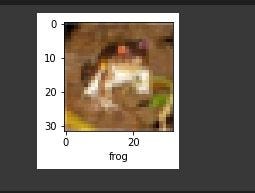
Then, we create the following function:

def plot_sample(X, y, index):
    plt.figure(figsize = (15,2))
    plt.imshow(X[index])
    plt.xlabel(classes[y[index]])

We can test the function as follows:

plot_sample(X_train, y_train, 0)

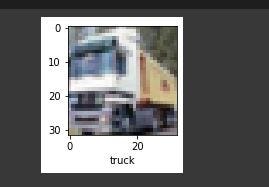
We can try another sample image:

plot_sample(X_train, y_train, 0)

Normalize the pictures to a value between 0 and 1. The image has three channels (R, G, and B), each of which can have a value between 0 and 255. So we must divide it by 255 to normalize it in the 0–1 range.

X_train = X_train / 255.0
X_test = X_test / 255.0

Model Building

We then construct an artificial neural network first, followed by a convolutional neural network, and we can test the effectiveness of both models as well as compare their benefits and drawbacks.

ann = models.Sequential([
        layers.Flatten(input_shape=(32,32,3)),
        layers.Dense(3000, activation='relu'),
        layers.Dense(1000, activation='relu'),
        layers.Dense(10, activation='softmax')    
    ])

ann.compile(optimizer='SGD',
              loss='sparse_categorical_crossentropy',
              metrics=['accuracy'])

ann.fit(X_train, y_train, epochs=5)

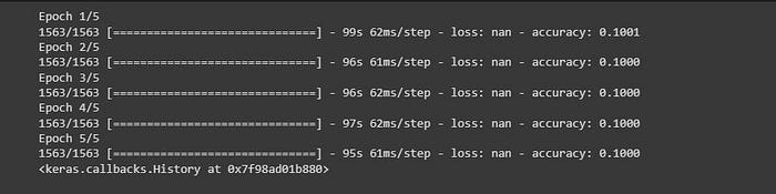
We can therefore see from the code above that there are four layers. The first layer accepts images with a 32 by 32 pixel dimension, while the second and third levels are deep layers with 3000 and 1000 neurons, respectively. The fourth layer then includes 10 categories to reflect the 10 sample images that are included in our dataset. After executing the code, we can see that the ANN’s accuracy on training samples is quite low—about 10%.

We then try it on test samples to see if the results get better.

ann.evaluate(X_test,y_test)

We can see from the review above that ANN continues to perform poorly. The last step is to print a classification report that displays the recall and precision for each sample image.

from sklearn.metrics import confusion_matrix , classification_report
import numpy as np
y_pred = ann.predict(X_test)
y_pred_classes = [np.argmax(element) for element in y_pred]

print("Classification Report: \n", classification_report(y_test, y_pred_classes))

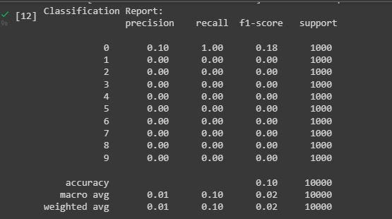
The precision and recall scores for each of the sample photos can then be examined (0–9). A sample image with index 1 has, for instance, the highest precision scores when compared to the others, as can be seen by looking at it.

The next step is to utilize build and train a CNN:

model = models.Sequential([
    layers.Conv2D(filters=32, kernel_size=(3, 3), activation='relu', input_shape=(32, 32, 3)),
    layers.MaxPooling2D((2, 2)),
    
    layers.Conv2D(filters=64, kernel_size=(3, 3), activation='relu'),
    layers.MaxPooling2D((2, 2)),
    
    layers.Flatten(),
    layers.Dense(64, activation='relu'),
    layers.Dense(10, activation='softmax')
])

model.compile(optimizer='adam',
              loss='sparse_categorical_crossentropy',
              metrics=['accuracy'])

We then run our loss and metrics tests using the Adam optimizer, which is known for its versatility.

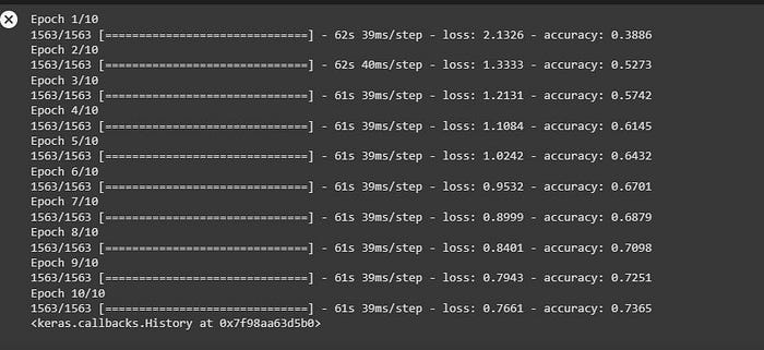
model.fit(X_train, y_train, epochs=10, verbose=1,batch_size=128)

We train the model for 10 epochs and get 70% accuracy, which is significantly higher than ANN.

To further our model building, we also try to evaluate the test dataset to see if we can get a high accuracy score.

model.evaluate(X_test,y_test)

The accuracy we have is 65%, which is above average, as we can then see.
So now that our CNN model is prepared, all that is left to do is plot a sample image and wait for the model to identify it.

plot_sample(X_test, y_test,6)

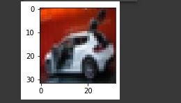
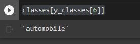
We can see that this is obviously an automobile; let’s see if our model can identify it as such.

classes[y_classes[6]]

Monitoring In Comet

In this section, I’ll be revealing the step-by-step process of logging our experiments in Comet.

The first step involves Installing comet which we have done at the beginning

!pip3 install comet_ml

The next step is to import experiments from Comet to enable us to log on to the Comet platform.

from comet_ml import experiment

We then move forward by creating an experiment and also setting the auto-logging features and other important features to true.

# Create an experiment
experiment = comet_ml.Experiment(
    project_name="image classification",
    workspace="<olujerry>",
     api_key="API_KEY",
    auto_metric_logging=True,
    auto_param_logging=True,
    auto_histogram_weight_logging=True,
    auto_histogram_gradient_logging=True,
    auto_histogram_activation_logging=True,
    log_code=True
)

The next step involves logging important features that we want to monitor on the Comet platform.

Using the experiment, we record some parameters using log_parameters(params):

batch_size = 128
epochs = 10
EMBEDDING_SIZE = 50
learning_rate = 0.001

params={
    "batch_size":batch_size,
    "epochs":epochs,
    "embed_size":EMBEDDING_SIZE,
    "optimizer":"Adam",
    "learning_rate":learning_rate,
    "loss":"sparse_categorical_crossentropy",
    }

experiment.log_parameters(params)

We then log the accuracy and loss of our model using the experiment.log_metric method:

loss, accuracy = model.evaluate(X_test,y_test)
print("Loss: ", loss)
print("Accuracy: ", accuracy)

experiment.log_metric("Loss", loss, step=None, include_context=True)
experiment.log_metric("Accuracy", accuracy, step=None, include_context=True)

Finally, before viewing our logged model on the Comet platform we log the saved model and then end the experiment afterward, as we are using an interactive notebook.

experiment.log_model(model, 'model')
experiment.end()

The next step involves checking out the performance of our model on the Comet platform.

Conclusion

We have successfully built a CNN model that helps classify images, and we also tested the ANN, and we were able to evaluate the efficiency of both models. Here is a link to my notebook, as well as the original notebook by Codebasics.