Introduction
3D Histograms or Ridge Plots are a great way to visualize the training progress of your Neural Network. Histogram distributions of the weights, gradients, and activations allow us to get some intuition for the loss surface that we are trying to optimize.
For example, your model may be approaching a local minima if you observe that your gradients are becoming smaller over time. On the flip side, a trend of large gradients with high variance might imply that you should reduce your learning rate, or use some form of regularization.
The Comet SDK provides an easy way to visualize your weights, activations and gradients using the `log_histogram_3D` method. For this post we will provide examples of histogram logging with Comet using Tensorflow’s Gradient Tape.
You can explore the visualizations in this post here. We have also included Colab Notebooks at the end of this post so that you can try out the histograms feature for yourself!
Logging Histograms
For this example, we are going to use a simple 2 layer perceptron and train it on the MNIST dataset. Let’s start by loading in our data, and defining our model
|
1
2
3
4
5
6
7
8
9
10
11
12
13
14
15
16
17
18
19
20
21
22
23
24
25
26
27
28
|
def get_dataset(): num_classes = 10 # the data, shuffled and split between train and test sets (x_train, y_train), (x_test, y_test) = mnist.load_data() x_train = x_train.reshape(60000, 784) x_test = x_test.reshape(10000, 784) x_train = x_train.astype("float32") x_test = x_test.astype("float32") x_train /= 255 x_test /= 255 print(x_train.shape[0], "train samples") print(x_test.shape[0], "test samples") # convert class vectors to binary class matrices y_train = to_categorical(y_train, num_classes) y_test = to_categorical(y_test, num_classes) return x_train, y_train, x_test, y_testdef build_model_graph(): model = Sequential() model.add(Dense(128, activation="sigmoid", input_shape=(784,), name="dense1")) model.add(Dense(64, activation="sigmoid", name="dense2")) model.add(Dense(10, activation="softmax", name="output")) return model |
Tensorflow’s GradientTape allows eager execution of model code without precomputing a static graph in which inputs are fed in through placeholders.
This implies that at every training step, we will have to calculate the gradients of our parameters with respect to our loss, and apply them with the optimizer in order to perform backpropagation.
|
1
2
3
4
5
6
7
8
9
10
11
12
|
def step(model, X, y, gradmap={}, activations={}): with tf.GradientTape() as tape: pred = model(X) loss = categorical_crossentropy(y, pred) grads = tape.gradient(loss, model.trainable_variables) opt.apply_gradients(zip(grads, model.trainable_variables)) gradmap = get_gradients(gradmap, grads, model) activations = get_activations(activations, X, model) return loss.numpy().mean(), gradmap, activations |
We will use two dictionaries to store layerwise information about the gradients and activations. For each batch of data we will accumulate the values of the gradients and activations. At the end of every epoch we will scale these by the number of batches in an epoch, and log them to Comet.
|
1
2
3
4
5
6
7
8
9
10
11
12
13
14
15
16
17
18
19
20
21
22
23
24
25
26
27
28
29
30
31
32
33
34
35
36
37
38
39
40
|
def train(model, X, y, epoch, steps_per_epoch, experiment): gradmap = {} activations = {} total_loss = 0 with experiment.train(): # show the current epoch number print("[INFO] starting epoch {}/{}...".format(epoch, EPOCHS), end="") for i in range(0, steps_per_epoch): start = i * BS end = start + BS curr_step = ((i + 1) * BS) * epoch loss, gradmap, activations = step( model, X[start:end], y[start:end], gradmap, activations, ) experiment.log_metric( "batch_loss", loss, step=curr_step ) total_loss += loss experiment.log_metric( "loss", total_loss / steps_per_epoch, step=epoch * steps_per_epoch ) # scale gradients for k, v in gradmap.items(): gradmap[k] = v / steps_per_epoch # scale activations for k, v in activations.items(): activations[k] = v / steps_per_epoch log_weights(experiment, model, epoch * steps_per_epoch) log_histogram(experiment, gradmap, epoch * steps_per_epoch, prefix="gradient") log_histogram(experiment, activations, epoch * steps_per_epoch, prefix="activation") |
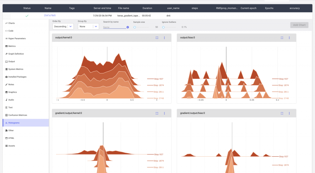
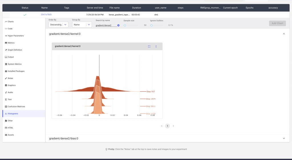
We can visualize these reported values under the Histograms tab in our Comet Experiment
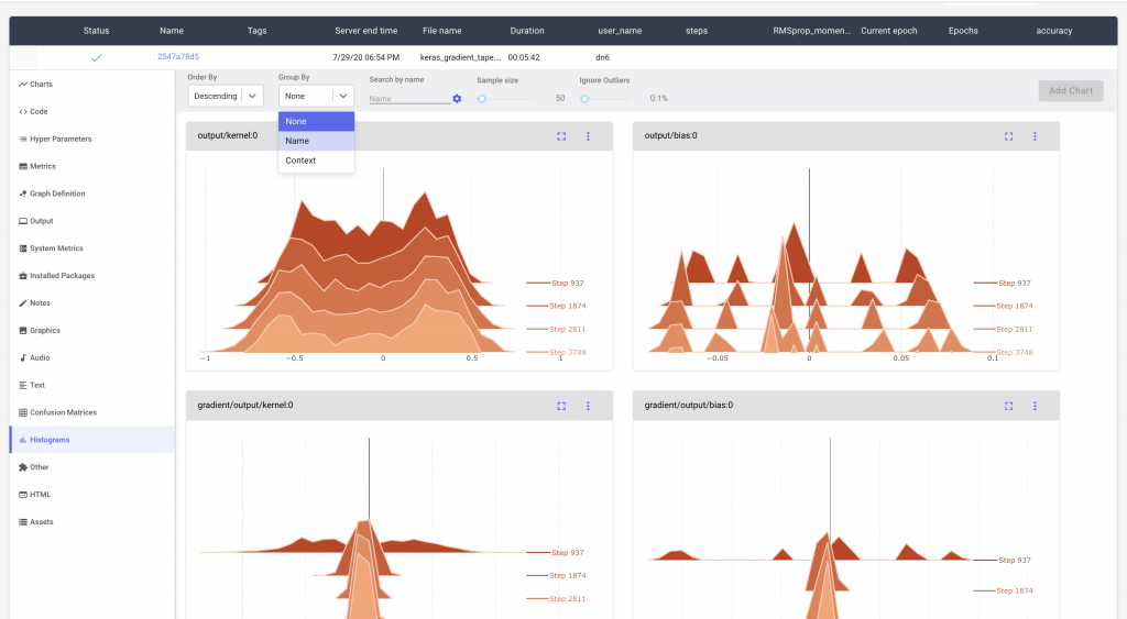
We can sort and search the various histograms using the options in the menu. For example, we might want to group our histograms based on the reported names
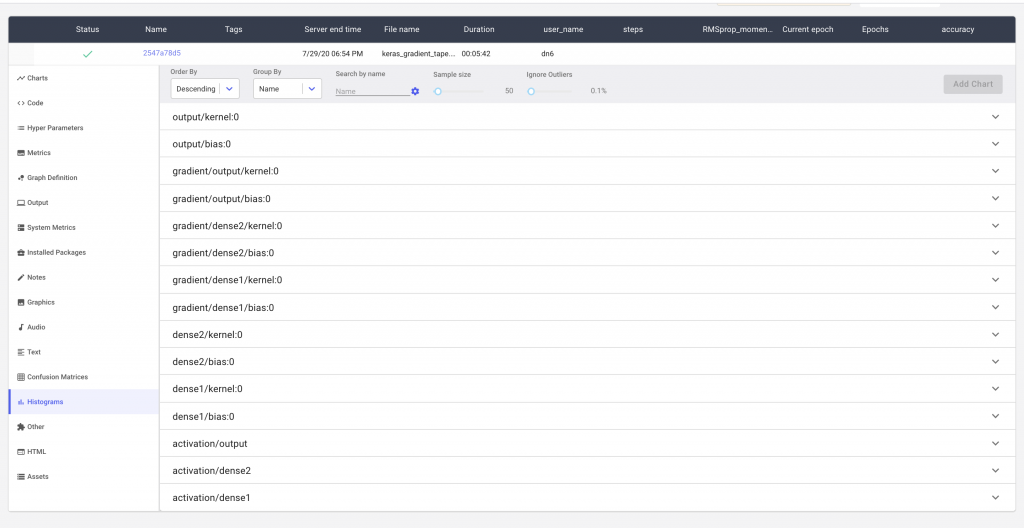
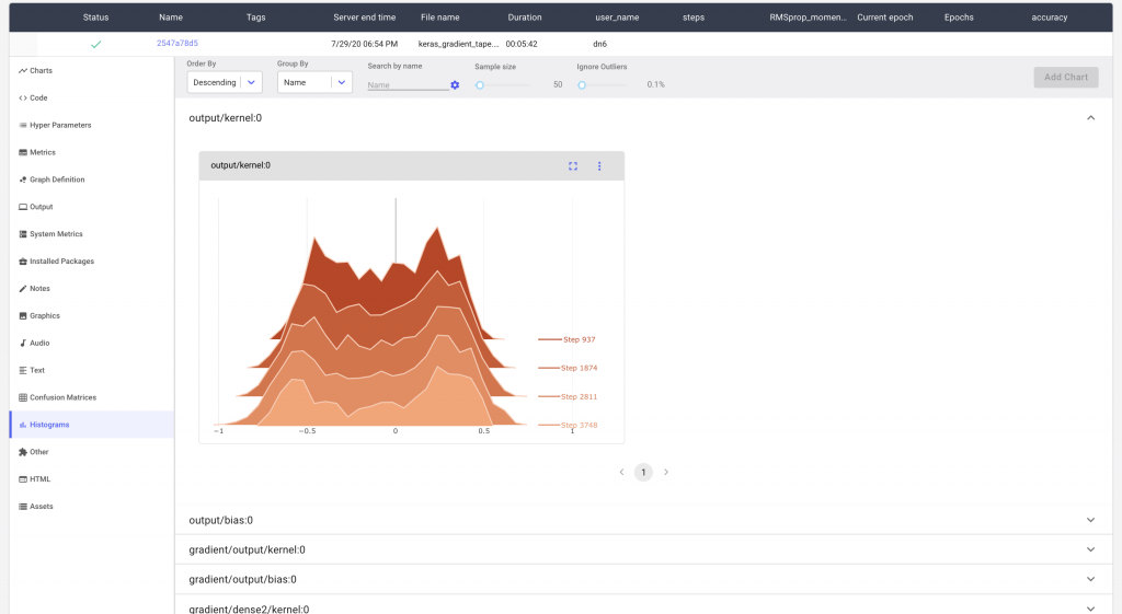
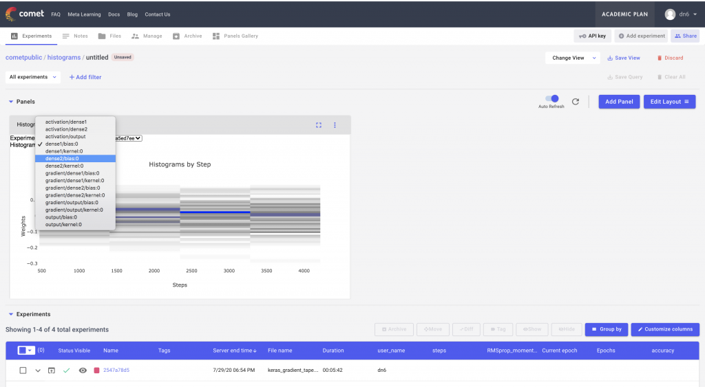
For larger models, we may have many such histograms. Comet makes it possible to search for the specific histogram that you’re interested in. In Figure 5 we can see how we are able to search for the histogram distribution of the gradients of a single layer.
Additionally, Comet provides Custom Panels that can visualize these histograms as a heatmap over time. This particular custom panel can be found in Panels Gallery → Public Panels → Histogram by Step. After adding the Panel to the project, we should see it above the Experiment Table.

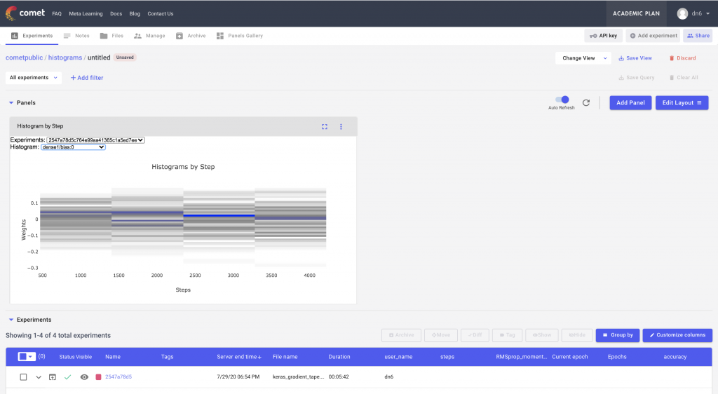
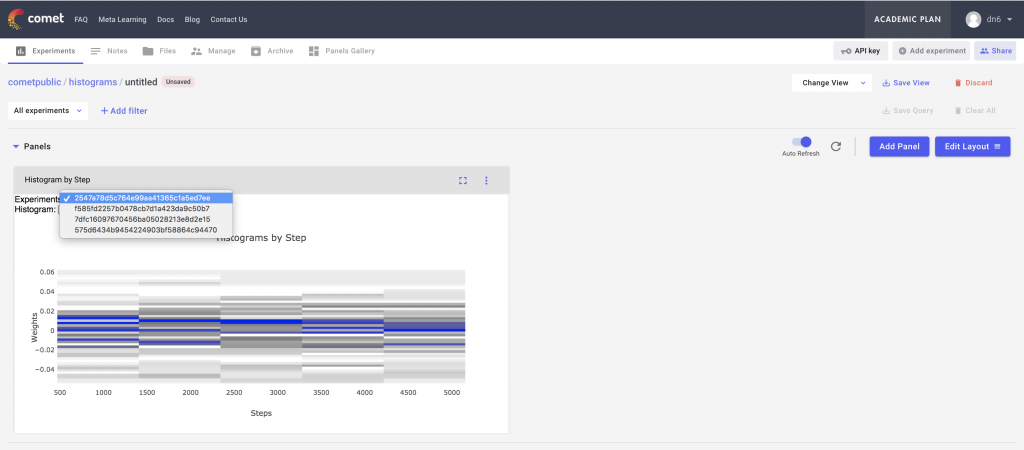
This custom panel has drop downs for both the experiment ids and the histogram names. We can select a particular experiment from the dropdown and then visualize the individual histograms in that experiment as a heat map over time.
Conclusion
In this post we demonstrated how Comet’s histogram logging and Custom Panels can be used to visualize the weights, gradients, and activations of a Neural Network.
Colab Notebooks :