Sometimes when you build a Machine Learning model, the results produced differ from those expected, despite having appropriately taken all the necessary precautions (feature selection, model optimization, and so on). In these cases, you move on to the troubleshooting phase, where, in addition to looking for any errors in the code, you can resort to so-called reverse engineering. Reverse engineering indicates starting with the results, and working backwards to try to understand how these results were produced.

There are several techniques for performing reverse engineering in the Machine Learning sector. In this article, I describe one, based on the calculation of the Shapley value, a metric that describes the contribution of each input feature to an algorithm in producing the final result.

There is a Python library that implements the Shapley value calculation, and also produces some interesting graphs. In this article I show how to use this library and how to integrate it into Comet.

Find the official documentation here.

The article is organized as follows:

• Quick overview of the Shapley Value
• A practical example

1. Quick overview of the Shapley Value

SHAP stands for SHapley Additive exPlanations. The concept of the Shapley value derives from cooperative game theory, and it measures the contribution of each player to a game.

In Machine Learning, a Shapley value measures the contribution of each input feature to the outcome, separately, as compared with all the other input features. In practice, a Shapely value permits understanding how a predicted value is built from the input features.

There is a Python library, named shap, which you can install through pip as follows:

pip install shap

The official documenation of the shap package is avalaible at this link.

To get started with the shap library, you should create an Explainer object, which receives as input a trained model:

import shap
explainer = shap.Explainer(model.predict)

Then, you can apply the created explainer to the dataset to test:

shap_values = explainer(X_test)

You can use the extracted shap values to plot different graphs, including summary plots, waterfall plots, and much more.

2. A practical example

As a practical example, we build a classification task, which uses the wine dataset, available at this link, and we track the results in Comet. The goal is to classify each wine, defined by some features, into one of the following two categories: red or white.

The example is organized as follows:

• setup of the environment
• loading and preparing the dataset
• training and evaluating the model
• calculating the Shapley value
• showing the results in Comet.

2.1 Setup of the environment

Firstly, we import all the required libraries:

from comet_ml import Experimentimport shap
shap.initjs()

*Note that we need to import the comet_ml library before the shap library.

Then, we create a file called .comet.config, which contains all the credentials used to access to Comet, and which is located in the same directory as that containing the scripting coding:

[comet]
api_key=YOUR_COMET_KEY
workspace=YOUR_WORKSPACE

Finally, we create the Comet experiment:

experiment = Experiment(project_name='wine-classification')
experiment.set_name('WineClassification')

2.2 Loading and preparing the dataset

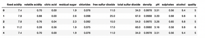
The original dataset is divided into two files, one for red wine, and the other for white wine. So, we load the dataset as two pandas dataframes:

import pandas as pddf_r = pd.read_csv('source/wine_quality/winequality-red.csv', sep=';')
df_w = pd.read_csv('source/wine_quality/winequality-white.csv', sep=';')
df_r.head()

We add a new line to each dataset, indicating the related label:

df_r['label'] = 'red'
df_w['label'] = 'white'

We merge the two datasets:

df = pd.concat([df_r, df_w])

We create the input and output variables:

X = df.drop("label", axis = 1)
y = df["label"]

We encode the labels:

from sklearn.preprocessing import LabelEncoderlabel_encoder = LabelEncoder()
y = label_encoder.fit_transform(y)

And we standardize input features:

from sklearn.preprocessing import StandardScalerscaler = StandardScaler()
X[X.columns] = scaler.fit_transform(X[X.columns])

And finally, we split data into training and test sets:

from sklearn.model_selection import train_test_split
X_train, X_test, y_train, y_test = train_test_split(X, y, test_size=0.10, random_state=42)

Comet Artifacts lets you track and reproduce complex multi-experiment scenarios, reuse data points, and easily iterate on datasets. Read this quick overview of Artifacts to explore all that it can do.

2.3 Training and evaluating the model

We will use a Gaussian Naive Bayes classifier for our model. We train it with the training set as follows:

from sklearn.naive_bayes import GaussianNBmodel = GaussianNB()
model.fit(X_train,y_train)

Now we calculate the accuracy of the model:

from sklearn.metrics import accuracy_score
y_pred = model.predict(X_test)
accuracy_score(y_test, y_pred)

The model reaches an accuracy of 0.9676923076923077.

2.4 Calculating the Shapley value

Firstly, we create an Explainer object as follows:

explainer = shap.Explainer(model.predict, X_train)
shap_values = explainer(X_train)

For some models you need to specify the model.predict function as an input parameter, for other models, you should specify only the model. For the Gaussian Naive Bayes classifier, we will be using model.predict.

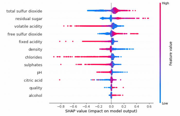
Then, I create the summary plot for the training dataset:

shap.summary_plot(shap_values, X_train)

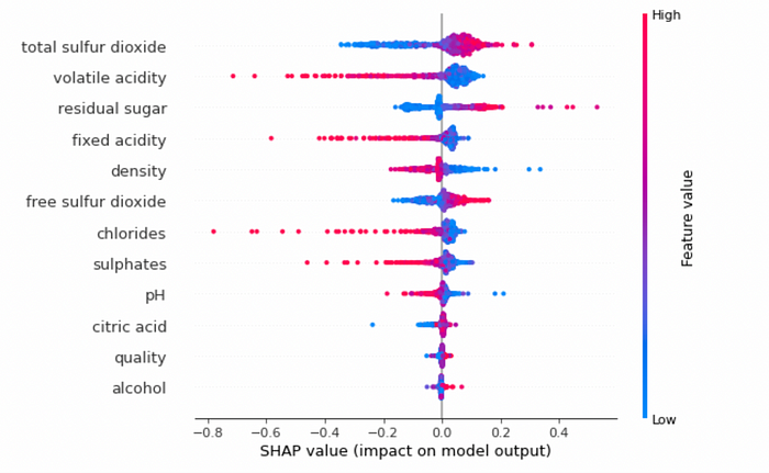
and also for the test set:

explainer = shap.Explainer(model.predict, X_test)
shap_values = explainer(X_test)
shap.summary_plot(shap_values, X_test)

2.5 Showing the results in Comet

After running the experiment, you will see the completed graphs in Comet, under the Graphics section, as shown in the following figure:

Summary

Congratulations! You have just learned how to integrate Shapley values in Comet! The procedure is very simple, because once you have created the experiment, Comet will log the produced graphs automatically.

You can download the code used in this article directly from this Github repository, as well as you can see the results directly in Comet here!

Happy coding! Happy Comet!