Integrating Comet and Azure Databricks

Introduction

Recently I made the switch to actively tracking my machine learning experiments. First with ML Flow and then with Comet.

Tracking experiments is becoming more common in MLOps. As time goes on, data scientists and machine learning engineers have realized the importance of model versioning. This has gone beyond saving metrics in experiments. Modern experiment tracking now includes saving metrics, logging charts, and even saving artifacts.

In this article, we’ll focus on Comet’s experiment tracking within an Azure Databricks environment. In this article I’ll cover four things:

• Setting Up Comet ML in Azure Databricks
• Creating an Experiment
• Using Comet for Exploratory Data Analysis
• Creating Algorithms and Comparing the Results in Comet

Databricks has built-in ML experiment tracking using MLFlow, which I find not very beginner friendly, with a high learning curve. Comet is easy to use for data science professionals of different skill levels and is easy to set up.

The goal of this project is to demonstrate for beginners the advantages of Comet in an Azure Databricks environment.

Installing Libraries in Azure Databricks

This article assumes you know how to navigate Databricks and upload/mount the datasets that will be used.

Dependencies:

• comet_ml
• comet-for-mlflow

Other libraries such as pandas, numpy, scikit-learn, Seaborn, and matplotlib are already pre-installed in Databricks.

Install Process

The installation process is straightforward for installing Comet into Azure Databricks. If you already use AutoML, installing the comet-for-mlflow package is also really useful. Comet will log your existing MLFlow work and save it to a current Comet experiment.

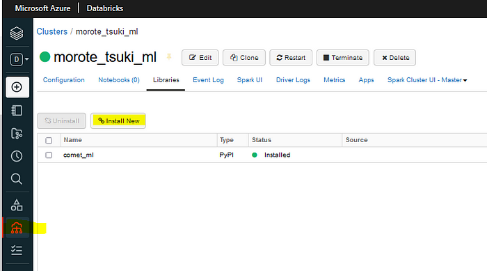
The first step is installing it in the cluster. Once you have started your cluster, select the Install New button, highlighted below.

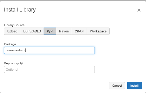
In the Install Library window, select PyPI. Then type the name of the package. I would recommend at this point installing both comet_ml and comet_automl.

There is an option to install on all your current clusters — this a personal choice. Generally, I only install Comet Libraries on either my clusters used for development or for production.

Since Databricks is not a Jupyter Notebook nor a Python file, there will be instances where certain Comet features do not work. You will often have to cover gaps with AutoML, depending on what you want to save to your experiments.

Now you’re ready to set up an experiment in a Databricks notebook.

Before we create the experiment, let’s first look at the dataset we will be using. The data set is the Diamonds dataset from Kaggle.

Data

The diamond data set has 53940 rows and 10 features:

• price — price in US dollars (numeric)
• carat — weight of the diamond (numeric)
• cut — quality of the cut (categorical)
• color — diamond color (categorical)
• clarity — a measurement of how clear the diamond is (categorical)
• x — length in mm (numeric)
• y — width in mm (numeric)
• z — depth in mm (numeric)
• depth — total depth (numeric)
• table — width of top of diamond relative to widest point (numeric)

Further information on carat, cut, color, quality, and other terms can be found here.

Creating an Experiment

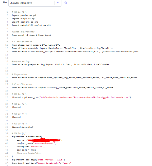
Before creating your experiment, select the computer cluster where you installed comet and comet_automl. Once you have selected the cluster, create a new Databricks notebook. We will load the following libraries:

import pandas as pd 
import numpy as np 
import seaborn as sns 
import matplotlib.pyplot as plt

#Comet Experiments 
from comet_ml import Experiment

# Classification
from sklearn.svm import SVC, LinearSVC
from sklearn.ensemble import RandomForestClassifier , GradientBoostingClassifier
from sklearn.discriminant_analysis import LinearDiscriminantAnalysis , QuadraticDiscriminantAnalysis

# Regression
from sklearn.linear_model import LinearRegression,Ridge,Lasso
from sklearn.ensemble import RandomForestRegressor,BaggingRegressor,GradientBoostingRegressor,AdaBoostRegressor 
from sklearn.svm import SVR
from sklearn.neighbors import KNeighborsRegressor
from sklearn.neural_network import MLPRegressor

# Modelling Helpers :
from sklearn.preprocessing import  Normalizer , scale
from sklearn.model_selection import train_test_split
from sklearn.feature_selection import RFECV
from sklearn.model_selection import GridSearchCV , KFold , cross_val_score

#preprocessing :
from sklearn.preprocessing import MinMaxScaler , StandardScaler, LabelEncoder

# Regression
from sklearn.metrics import mean_squared_log_error,mean_squared_error, r2_score,mean_absolute_error 

# Classification
from sklearn.metrics import accuracy_score,precision_score,recall_score,f1_score

Once you have loaded the libraries, load your dataset into Databricks. You can do this by uploading your CSV directly to Databricks. If you have a blob storage, you can mount the storage container.

Setting Up an Experiment

Let’s create an experiment. When you first create your experiment, make sure you add the API key from your Comet account. The Comet account name is your workspace name, so add it as well.

Once you have added it, add your experiment name. This will be the main repository for all the runs in your experiment. If the experiment name does not exist in your Comet workspace, it will create a new experiment with the name.

If you want your code to show in a run, then set log_code parameter to True. If you are concerned about privacy or revealing your IP address, set log_env_host to False. Azure will log different environment settings than if you ran it in a Jupyter Notebook.

For the sake of clarity, I always add an experiment tag to note the experiment environment. I also add tags for experiment models that are in development, staging, and production.

If you are working in a team, you may not be working solely in Databricks, so it helps to add multiple tags.

What tips do big name companies have for students and start ups? We asked them! Read or watch our industry Q&A for advice from teams at Stanford, Google, and HuggingFace.

EDA in Databricks

Exploratory data analysis using Comet in Azure Databricks works very similar to using it in a Jupyter Notebook.

Logging figures is pretty important. Data may change between runs of an experiment for various reasons, so it’s important to save charts from your EDAs to an experiment.

To be able to create the figures, your dataframe will need to be in a pandas format rather than in a Spark dataframe.

Logging Figures

In Comet there are two ways to log figures to an experiment: matplotlib or seaborn. For this project, we used both Seaborn and matplotlib.

An example of logging a matplot lib figure is here:

plt.plot(diamond['carat'], diamond['price'], '.')
plt.xlabel('carat')
plt.ylabel('price')
experiment.log_figure(figure=plt)

Matplotlib is the simplest way to log a graph. Simply put the experiment.log_figure method after your completed figure. Do not add the plt.show()—you will get an error and the figure will not be saved.

Unlike matplotlib, Seaborn has some trouble saving charts in Comet. There’s a quick workaround to this. You will first need to save the Seaborn figure as a variable. Then convert it using .fig or .figure — some charts can only be saved using one of these.

I used the following method to save the charts:

def log_SeaFigure(fig, fig_name):
    '''
    Logs the seaborn figure, first by using depreciated ax.fig, and runs ax.figure if an exception is raised. 
    
    Parameters: 
    fig (object) - seaborn figure
    fig_name (string) - the user defined name for seaborn figure in comet experiment 
    
    Returns: 
    Logs figure to comet experiment log, and prints the method used or an error message. 
    
    '''
    ax = fig
    try:
      experiment.log_figure(fig_name, ax.fig)
      print('Log Figure Successful using ax.fig')
    except: 
      experiment.log_figure(fig_name, ax.figure)
      print('Log Figure Successful using ax.figure')
    else:
      print("Figure Error: Please check chart parameters")

Alternatively, you can use exception handling without using the method:

ax = sns.violinplot(x="cut",y="price",data=df2)

try:
      experiment.log_figure(fig_name, ax.fig)
      print('Log Figure Successful using ax.fig')
except: 
      experiment.log_figure(fig_name, ax.figure)
      print('Log Figure Successful using ax.figure')

For this article we also logged histograms, a correlation matrix and a scatter plot, and a violin plot. Let’s take a look at the figures that we logged in our test EDA.

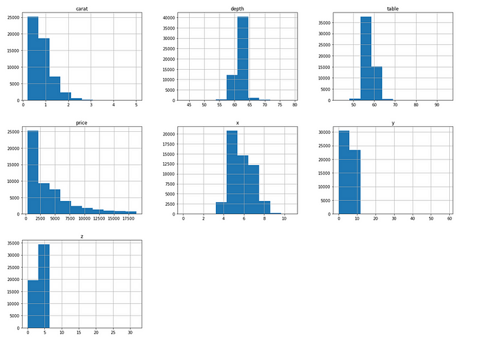
Histograms

In the dataset, diamonds usually have smaller carat size and prices. The length, width, and height (x,y,z) are within very small ranges.

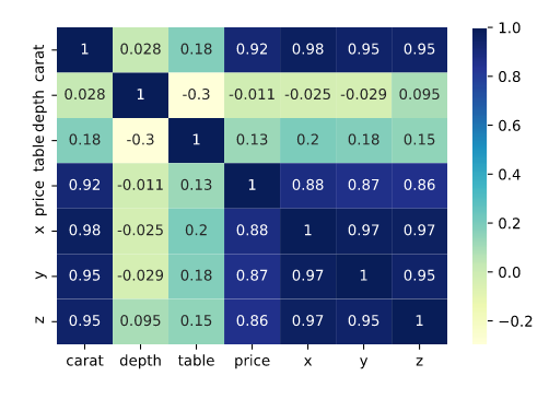
Correlation Matrix

Carat, width, depth, and height are highly correlated with each other. Price is also highly correlated with carat size. Given their high correlation with each other, they may be multi-collinear. We will be dropping these variables later down the line.

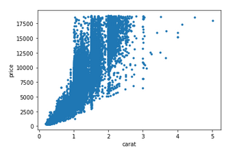
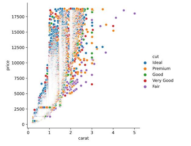
Carat vs. Price

As we can see from the model, most cuts range from below 1 carat to 2.5 carats, regardless of cut quality. This suggests that the carat size is being standardized.

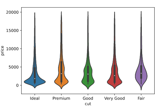
Cut vs. Price

The median price for all cuts is below $5000 USD. Ideal cuts show the lowest median price. Premium, good, and fair cuts have a higher median price than very good and premium cuts.

Model Preparation

To prep for modeling we first have to do three steps: transforming the data, converting the dataframe to Spark, and vectorizing.

Data Transformation

The dataset still contains three categorical features: cut, color, and clarity. In addition, it contains three variables: length(x), width (y), and depth (z).

We will first encode the categorical variables since we cannot use string data types for vector encoding features. We will also drop the x, y, and z. An example of this is below:

#Feature Endcode Using a Dictonary
diamond['cut'] = diamond['cut'].replace({'Fair':0, 'Good':1, 'Very Good':2, 'Premium':3, 'Ideal':4})
diamond['color'] = diamond['color'].replace({'J':0, 'I':1, 'H':2, 'G':3, 'F':4, 'E':5, 'D':6})
diamond['clarity'] = diamond['clarity'].replace({'I1':0, 'SI1':1, 'SI2':2, 'VS1':3, 'VS2':4, 'VVS1':5, 'VVS2':6, 'IF':7})

#Drop length, width, and depth columns 
diamond.drop(['x','y','z'], axis=1, inplace= True)

Now that that’s done, let’s convert the panadas dataframe to a Spark dataframe.

Converting Dataframe to Spark

Vectorizing

The second step is vectorizing. We do this using VectorAssembler. This method is a transformer that combines a given list of columns into a single vector column, which is added to the data frame.

Vectorization is useful for combining raw features and features generated by different feature transformers into a single feature vector in order to train ML models like logistic regression and decision trees.

The code example is below:

#Transform all features into output column named "features"
vectorAssembler = VectorAssembler(inputCols = ['carat', 'cut', 'color', 'clarity', 'depth', 'table'], outputCol = 'features')
vdiamond_df = vectorAssembler.transform(spark_diamond_drop) #adds feature to spark_diamond_drop df 

#Creates a df from features column and the target variable 
vdiamond_df = vdiamond_df.select(['features', 'price'])

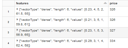
Once we vectorized the features ‘carat,’ ‘cut,’ ‘color,’ ‘clarity,’ ‘depth,’ and ‘table,’ we will select only the price (our target variable) and the features column created by the VectorAssembler method into a new dataset.

The dataset should look like this after selecting only the features and price columns:

Now that we have created the data frame, we will split it randomly into testing and training datasets. In PySpark, this is done using the random split method:

splits = vdiamond.randomSplit([0.7, 0.3])
train_df = splits[0]
test_df = splits[1]

Now that we have split the data into train_df and test_df, it’s time to build the models.

Building the Algorithms

To keep it simple, I will be focusing on linear regression. The three models that we will be creating are ordinary least squares, decision tree regression, and gradient boosted regression. Since Databricks is a Spark environment, we will be using PySpark to create these algorithms.

PySpark has its own built-in library for machine learning, pyspark.ml.regression. From this library we imported the LinearRegression, RegressionTree, and GBTRegressor methods.

For each regression we created the algorithm, labeled the features column, then logged the metrics to a variable, which we uploaded to our Comet experiment.

The methods to obtain metrics for decision tree regression and gradient boosted regressor are different than linear regression. So we created a method called get_SparkMetric to obtain the metrics for each:

def get_SparkMetric(labelCol, predCol, metricName, dfPrediction):
    '''
    Returns the a user-specified statistical metric for non-linear regression
    
    Parameters: 
    labelCol (str) - target column of a Spark Regression 
    predCol (str) - predicted values of regression 
    metricName (str) - metric used for model, such as RMSE, MAE, R2, MSE
    dfPrediction (obj) - transformed dataframe from test data 
    
    Returns: 
    Metric value for regression 
    
    '''
    evaluator = RegressionEvaluator(labelCol=labelCol, predictionCol=predCol, metricName=metricName)
    metric = evaluator.evaluate(dfPrediction)
    return metric

The metrics we will be logging are:

• R2 (Fit)
• Mean Square Error (MSE)
• Root Mean Square Error (RMSE)
• Mean Absolute Error (MAE)

For each of the metrics, we will use the experiment.log_metric method. This method will log a value for each to metric a given experiment run. The method also allows you to set the name of the metric in the experiment store.

Now, let’s look at the regression types we will be using.

Innovation and academia go hand-in-hand. Listen to our own CEO Gideon Mendels chat with the Stanford MLSys Seminar Series team about the future of MLOps and give the Comet platform a try for free!

Linear Regression

To get metrics for linear regression, we need to do the following:

• Create the linear regression model and specify the feature column and our label columns.
• Fit the model to the training data frame.
• Run and summarize the model metrics using .summary.
• After loading into a variable, we call the metrics.

An example is below:

#Linear Regression Model 
from pyspark.ml.regression import LinearRegression
lr = LinearRegression(featuresCol = 'features', labelCol='price', maxIter=10, regParam=0.3, elasticNetParam=0.8)
lr_model = lr.fit(train_df)

#Save metrics to variables
lr_trainingSummary = lr_model.summary
lr_r2 = lr_trainingSummary.r2
lr_mse = lr_trainingSummary.meanSquaredError
lr_rmse = lr_trainingSummary.rootMeanSquaredError
lr_mae = lr_trainingSummary.meanAbsoluteError

#Log Metric to Comet Experiment
experiment.log_metric("LR_r2", lr_r2, step=0)
experiment.log_metric("LR_MSE", lr_mse, step=0)
experiment.log_metric("LR_RMSE", lr_rmse, step=0)
experiment.log_metric("LR_MAE", lr_mae, step=0)

#Display Metrics 
print("RMSE: %f" % lr_r2)
print("MSE = %s" % lr_mse)
print("r2: %f" % lr_rmse)
print("MAE = %s" % lr_rmse)

The model logs the following metrics:

• RMSE: 0.892751
• MSE = 1707708.8
• r2: 1306.793,
• MAE = 1306.7933613787445

Decision Tree

With decision tree regression, we need to import both the DecisionTreeRegressor and RegressionEvaluator. We will be using the last one to get the metrics since the .summary method is used only with linear regression.

To simplify the code we used the get_SparkMetric method detailed earlier in the article. The method is used to gather the metric from the model which is then logged into the experiment run.

An example of this is shown below:

from pyspark.ml.regression import DecisionTreeRegressor
from pyspark.ml.evaluation import RegressionEvaluator #This is needed to run the get_SparkMetric function. 

#create and fit model
dt = DecisionTreeRegressor(featuresCol ='features', labelCol = 'price')
dt_model = dt.fit(train_df)
dt_predictions = dt_model.transform(test_df)

#create metrics
dt_r2 = get_SparkMetric("price", "prediction", "r2", dt_predictions)
dt_rmse = get_SparkMetric("price", "prediction", "rmse", dt_predictions)
dt_mae = get_SparkMetric("price", "prediction", "mae", dt_predictions)
dt_mse = get_SparkMetric("price", "prediction", "mse", dt_predictions)

#log metrics 
experiment.log_metric("dt_r2", dt_r2, step=0)
experiment.log_metric("dt_rmse", dt_rmse, step=0)
experiment.log_metric("dt_mae", dt_mae, step=0)
experiment.log_metric("dt_mse", dt_mse, step=0)

The model returns the following metrics:

• RMSE: 0.892751
• MSE = 1707708.8
• r2: 1306.793,
• MAE = 1306.7933613787445

Gradient Boosted Regressor

Gradient boosted regressor’s metrics are recorded in the same way as the decision tree model, using the get_SparkMetric.

from pyspark.ml.regression import GBTRegressor
from pyspark.ml.evaluation import RegressionEvaluator #This is needed to run the get_SparkMetric function.

#create and fit model 
gbt = GBTRegressor(featuresCol = 'features', labelCol = 'price', maxIter=10)
gbt_model = gbt.fit(train_df)
gbt_predictions = gbt_model.transform(test_df)

#create metrics
gbt_r2 = get_SparkMetric("price", "prediction", "r2", gbt_predictions )
gbt_rmse = get_SparkMetric("price", "prediction", "rmse", gbt_predictions)
gbt_mae = get_SparkMetric("price", "prediction", "mae", gbt_predictions)
gbt_mse = get_SparkMetric("price", "prediction", "mse", gbt_predictions
                          
#log metrics
experiment.log_metric("gbt_r2", gbt_r2, step=0)
experiment.log_metric("gbt_rmse", gbt_rmse, step=0)
experiment.log_metric("gbt_mae", gbt_mae, step=0)
experiment.log_metric("gbt_mse", gbt_mse, step=0)

print("r2: %f" % gbt_r2)
print("MSE = %s" % gbt_mse)
print("RMSE: %f" % gbt_rmse)
print("MAE = %s" % gbt_rmse)

The model returns the following metrics:

• RMSE: 0.892751
• MSE = 1707708.8
• r2: 1306.793,
• MAE = 1306.7933613787445

Once you have logged the metrics to the run, end the experiment by creating a cell with experiment.end() . The end result should look like the picture below:

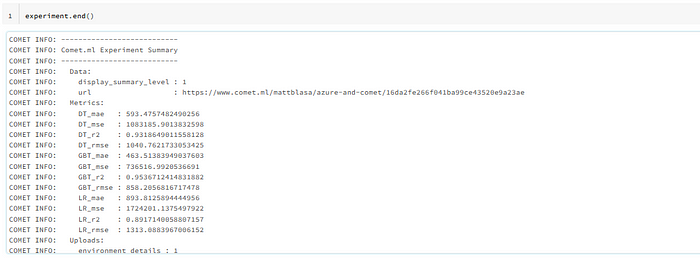
After you have done that, let’s check out the results in Comet. The url displayed at the end of the run is the location of your experiment in your Comet workspace.

Comparing the Results in Comet

Let’s check how the experiment logged the data and how the metrics compared to each other. The data saved in each experiment can be used to check for subtle changes in the model, metrics, and even the dataset.

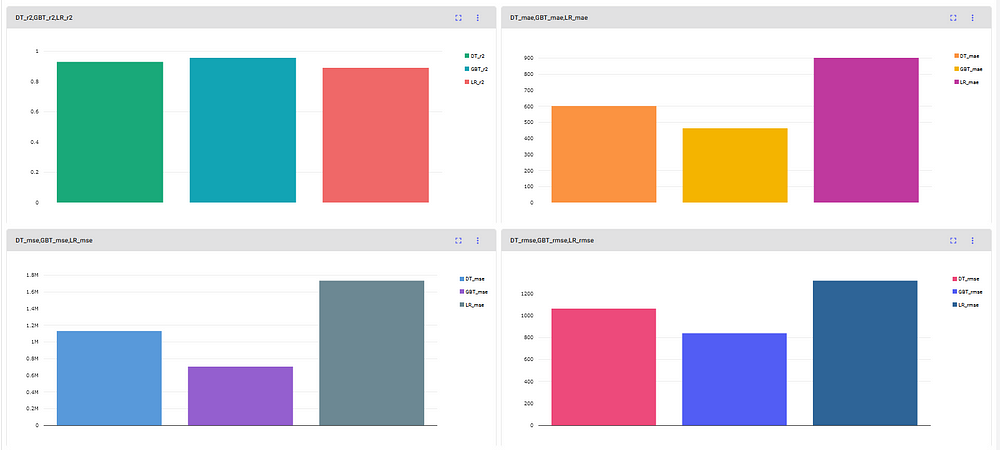
Let’s now look inside the Panels tab (i.e., Comet’s concept for data visualization).

Panels

We separated the metrics into four distinct graphs comparing the r2, mean squared error, mean absolute error, and root mean square error. The gradient boost out-performed simple linear regression and regression tree.

Metrics

You can also view the logged metrics in the metrics tab. The metrics tab also includes features that allow you to search by metric name and change the decimal precision.

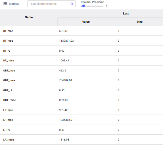
From both the charts and metric data, the gradient boosting algorithm performed the best compared to simple linear regression and regression tree.

Charts

If we want to look at the charts we created from the EDA we need to click the graphics tab of the experiment. The Seaborn and matplotlib figures will be saved in the experiment. We can search for these figures by the name we assigned when we logged the figures.

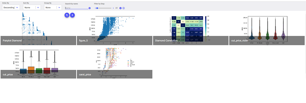
Saving these charts is really valuable, especially if you need to create reports or presentations for stakeholders. It’s also quite useful if another teammate is attempting to replicate the results of your EDA on their own computer.

Now, let’s check out my favorite Comet feature: Code Logging.

Code Logging

The Azure Databricks environment doesn’t integrate with GitHub like a Jupyter Notebook would (sad, I know). However, it does log the code from your Databricks notebook if you set it up in the initial experiment.

The code inside the experiments can be accessed from the code tab in the Comet UI.

All the code between the experiment() method and the experiment.end() method will be logged. Any code that is outside these blocks will not be logged. The tab also allows you to export your code via the download button in the upper right corner.

Conclusion

Well, that’s it! You’ve successfully logged your first experiment in Comet using Azure Databricks. Databricks is a different environment combined with Comet, and can really speed up your experiment tracking.

Links to my Github repository and Comet Experiment repository are below:

• GitHub Repository
• Comet Experiment Log

Thank you for reading! Connect with me on LinkedIn for more on data science topics.