Computer vision is an interesting field in machine learning as it helps computers understand what they see. Computer vision has various sub-topics like segmentation, object detection, image synthesis, etc. This tutorial will focus on building image classifiers from the ground up and monitoring the training process.

Image classification is a computer vision task that allows algorithms to understand an image’s contents and assign one or more categories to the image. Image classifiers are considered the basis of other computer vision problems. It can be used in a wide range of applications, especially when used with the Internet of Things. Examples of applications of image classification include:

• Automated inspection and quality control in production and manufacturing industries.
• Detection of plant diseases and improve quality of produce in farms.
• Traffic monitoring to help de-congest cities.
• Identifying diseases in medical images like X-Rays or CT-Scans.

In this tutorial, you will use the Fashion MNIST dataset that contains 72K grayscale images of clothes belonging to 10 categories.

Pre-requisites

To follow along with this tutorial, you need to make sure your development environment is set up as follows:

• Install R binaries from their Official Website.
• After installing R, install R Studio, the preferred IDE coding R projects.
• Sign up for a free account to use Comet ML’s platform.

Getting Started

Let’s install some dependencies that you need to build your image classifier. You will install all these dependencies by using R Studio. Open R Studio and, in the console, type in the following commands to install the dependencies needed.

First, install Comet’s R package which will be used to log metrics to your Comet account

install.packages(“cometr”)

Next, you will need to install the Keras package for R by running the following command in the console. Keras provides a simple API to build neural networks and uses Tensorflow as the backend.

install.packages(“keras”)

Now you have your development environment set up. Let’s begin by loading the datasets.

Data Loading

The Fashion MNIST dataset can be accessed directly from Keras. Create a new R Script and call it image-classifer.R. This script file will host all the source code outlined in this tutorial. First load the R packages needed to run this project.

library(keras)
library(cometr)
library(tidyr)

To download the Fashion MNIST dataset, add the following code to your R script. You will use 60K images to train your model and 10K to evaluate the accuracy of your model.

fashion_mnist <- dataset_fashion_mnist()
c(train_images, train_labels) %<-% fashion_mnist$train
c(test_images, test_labels) %<-% fashion_mnist$test

The train_images and train_labels arrays are the training set and the test_images and test_labels are the testing set. The images are each 28 x 28 arrays, with pixel values ranging from 0 to 255. The labels are arrays of integers ranging from 0 to 9, representing the class of the clothing item the image represents.

Add the following vector to represent the class names since they are not included in the dataset.

class_names = c('T-shirt/top', 'Trouser', 'Pullover', 'Dress', 'Coat', 'Sandal', 'Shirt', 'Sneaker', 'Bag', 'boot')

Before building the model, we need to pre-process the data. For the image data, the pixel values range from 0 to 255. Before feeding these values to a neural network, the pixel values need to range from 0 to 1.

train_images <- train_images / 255
test_images <- test_images / 255

Have you tried Comet? Sign up for free and easily track experiments, manage models in production, and visualize your model performance.

Training the Neural Network

In this section, you will build a neural network that requires configuring the layers of the model. For this tutorial, let’s keep it simple and create a network with three layers. Building a neural network with Keras is easy due to its simple API.

model <- keras_model_sequential()
model %>%
layer_flatten(input_shape = c(28, 28)) %>%
layer_dense(units = 128, activation = 'relu') %>%
layer_dense(units = 10, activation = 'softmax')

The first layer, layer_flatten, transforms the two-dimensional array of 28×28 pixels that represents the images to a one-dimensional array of 28*28 = 784 pixels. This layer is only responsible for reformatting the data and has no learning parameters.

The second and third layers are dense layers that are fully connected. The second layer has 128 nodes (or neurons) with a relu activation function. The third layer is a 10-node softmax layer that returns the probability scores that the current image belongs to one of the 10 categories.

Loss Function & Optimizers

This section demonstrates how to add loss functions and optimizers to your neural network. Because the output of the network is a probability score of multiple categories, you can use a sparse categorical cross-entropy loss function. Add the following code block to your R script.

model %>% compile(
  optimizer = 'adam',
  loss = 'sparse_categorical_crossentropy',
  metrics = c('accuracy')
)

Monitoring

Before you start training, you’ll need to integrate Comet ML’s R package by adding the following code block. Ensure you have your API key from your Comet ML account, then create a .comet.yml file in your working directory. Follow the official documentation for additional help with getting started with R.

COMET_WORKSPACE: YOUR_COMET_USER_NAME
COMET_PROJECT_NAME: YOUR_PROJECT_NAME
COMET_API_KEY: YOUR_COMET_API_KEY

Next, create an experiment as shown below in your R script.

exp <- create_experiment(
  keep_active = TRUE,
  log_output = TRUE,
  log_error = FALSE,
  log_code = TRUE,
  log_system_details = TRUE,
  log_git_info = TRUE
)

Finally, you need to specify the number of epochs you want to train the network and log it using Comet ML.

epochs <- 20
exp$log_parameter("epochs", epochs)

Training

Now, train the model using the training datasets created above. First, let’s create a custom function to log losses to Comet ML after each step. This will help you visualize your experiments later on.

LogMetrics <- R6::R6Class("LogMetrics",
  inherit = KerasCallback,
  public = list(
    losses = NULL,
    on_epoch_end = function(epoch, logs = list()) {
      self$losses <- c(self$losses, c(epoch, logs[["loss"]]))
    }
  )
)
callback <- LogMetrics$new()

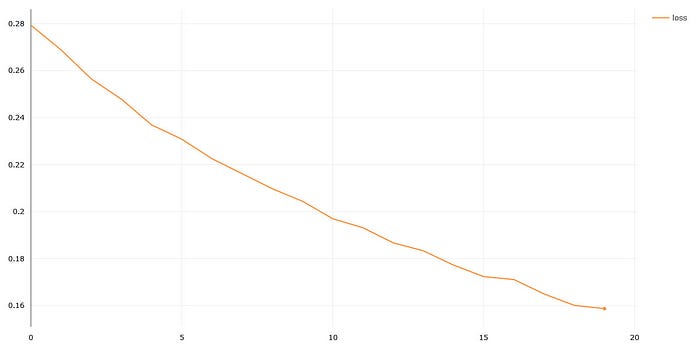
Next, train the model, and log your model’s loss after each step. This will create visualizations on your Comet account as shown below.

model %>% fit(train_images, train_labels, epochs = epochs, verbose = 2,
      callbacks = list(callback))
losses <- matrix(callback$losses, nrow = 2)
for (i in 1:ncol(losses)) {
  exp$log_metric("loss", losses[2, i], step=losses[1, i])
}

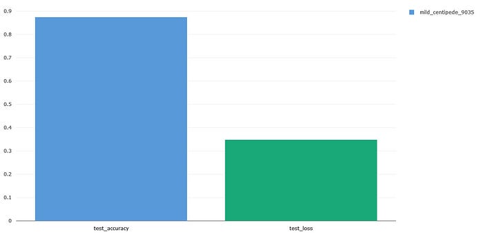
Make sure you log the training loss and accuracy metrics to Comet ML.

score <- model %>% evaluate(test_images, test_labels, verbose = 0)
exp$log_metric("test_loss", score["loss"])
exp$log_metric("test_accuracy", score["accuracy"])

You can now use your model to make predictions

predictions <- model %>% predict(test_images)

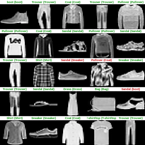
Finally, you want to see how your model classifies images in your test data. Let’s classify 25 images using our newly created model. Comet ML can upload the results of your experiments as artifacts as shown below.

png(file = "CompVisResults.png")

par(mfcol=c(5,5))
par(mar=c(0, 0, 1.5, 0), xaxs='i', yaxs='i')
for (i in 1:25) {
  img <- test_images[i, , ]
  img <- t(apply(img, 2, rev))
  predicted_label <- which.max(predictions[i, ]) - 1
  true_label <- test_labels[i]
  if (predicted_label == true_label) {
    color <- '#008800'
  } else {
    color <- '#bb0000'
  }

  image(1:28, 1:28, img, col = gray((0:255)/255), xaxt = 'n', yaxt = 'n',
        main = paste0(class_names[predicted_label + 1], " (",
                      class_names[true_label + 1], ")"),
        col.main = color)
}

dev.off()
exp$upload_asset("CompVisResults.png")

Conclusion

In this article, you’ve learned how to use Keras with R to build a neural network that can classify images into 10 categories. In addition, we logged some metrics like loss, accuracy, and epochs to Comet ML’s platform.

This tutorial was just a simple introduction to how to use R to build image classification models while monitoring your experiments using Comet ML. To improve the model’s accuracy, you can use data augmentation techniques to introduce randomness in the data and avoid over-fitting. Kindly visit Comet ML’s Official Documentation to gain more insights on how to monitor your R projects.