Photo by Graphic Node on Unsplash

Very deep neural networks can suffer from either vanishing or exploding gradients. This is because the main operation used to compute the derivatives as we propagate through a neural network model is matrix multiplication — thus, a network of n hidden layers will multiply n derivatives together.

When the derivatives are large, the gradient will increase exponentially as we propagate through the model until it eventually explodes. In contrast, when the derivatives are small, the gradient will decrease exponentially as we propagate through the model until it eventually vanishes. Both scenarios lead to the same end (in different ways): the network failing to learn well.

A partial solution to this problem is to be more careful when randomly initializing the weights of the network. This procedure is called weight initialization. The end goal of weight initialization is to prevent gradients from exploding or vanishing, thus, permitting a slightly more effective optimization process. It doesn’t entirely solve the vanishing/exploding gradient problem, but it’s an important design choice and helps a lot when building deep neural networks.

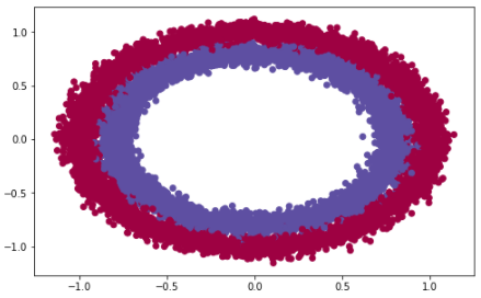
Let’s consider the make_circles dataset from scikit learn:

import numpy as np
import pandas as pd
import matplotlib.pyplot as plt
from sklearn.datasets import make_circles
from sklearn.model_selection import train_test_splitimport tensorflow as tf
from mlxtend.plotting import plot_decision_regionsimport warnings
warnings.filterwarnings("ignore")# load data
X_train, y_train = make_circles(n_samples=10000, noise=.05)
X_test, y_test = make_circles(n_samples=100, noise=.05)# visualize data
plt.subplots(figsize=(8, 5))
plt.scatter(X_train[:, 0], X_train[:, 1], c=y_train, cmap=plt.cm.Spectral)plt.show()

We are going to build a 4 layer neural network and test how it performs with different weight initializations. The full code for this notebook can be found via Github.

Zero Initialization

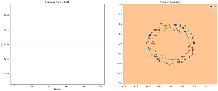
Zero initialization is exactly how it sounds: all weights are initialized as 0. In such scenarios, the neurons in each layer would learn exactly the same thing. Our network would fail to break symmetry as a consequence.

We can take this a step further and say: “whenever a constant value is used to initialize a model’s weights, you can expect it to perform poorly.” This is because the outputs of all hidden units in the model would have the same influence on the cost, thus, resulting in identical gradients.

Here’s the results of our model when we initialized weights as zero.

Tips, tricks, and innovation — all in your inbox each week. Subscribe to the Comet newsletter for the latest industry news gathered by our team of experts.

Random Initialization

Assigning weights random values breaks the symmetry. It’s better than zero but it’s not without some issues. Weights must not be initialized too high or too low because:

• If weights are initialized with large values then each matrix multiplication will result in a significantly larger value. Thus, applying a sigmoid activation function to the linear equation would result in a value close to 1 which slows down the rate of learning.
• If weights are initialized with small values then each matrix multiplication will result in significantly smaller values. Thus, applying a sigmoid activation function to the linear equation would result in a value close to 0 which slows down the rate of learning.

When initialized poorly, random initialization can lead to vanishing/exploding gradients. Let’s set the weights of our model to large values and see what happens:

def random_normal_init(shape, dtype=None):
return tf.random.normal(shape) * 1000model = tf.keras.Sequential([
tf.keras.layers.Dense(5, activation="tanh", input_shape=(X_train.shape[1],), kernel_initializer=random_normal_init),
tf.keras.layers.Dense(10, activation="tanh"),
tf.keras.layers.Dense(2, activation="tanh"),
tf.keras.layers.Dense(1, activation="sigmoid")
])model.compile(optimizer=tf.keras.optimizers.SGD(learning_rate=0.01),loss="mse", metrics=["accuracy"])history = model.fit(X_train, y_train, epochs=100, validation_data=[X_test, y_test])

Visualizing cost per epoch and decision boundary for a model with weights initialized from a random normal distribution.

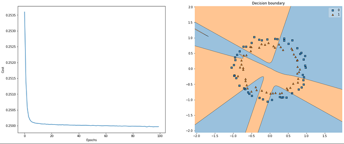
If we trained the algorithm longer, the results may have improved but initializing weights with large random values slows down optimization.

Xavier Initialization

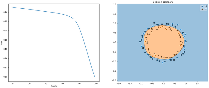
Xavier initialization also referred to as Glorot initialization, is a heuristic used to initialize weights. It’s become the standard way of initializing weights when the nodes either use tanh or sigmoid activation functions. It was first proposed in a paper by Xavier Glorot and Yoshua Bengio in 2010. The goal of Xavier initialization is to initialize weights such that the variance across layers in the network is the same. This helps to prevent the gradients from exploding or vanishing.

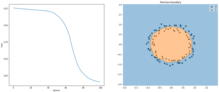
Here’s how our algorithm performed when we initialized our weights using Xavier uniform initialization:

Visualizing cost per epoch and decision boundary for a model with weights initialized with Xavier/Glorot uniform distribution.

He Initialization

He/Kaiming initialization is another heuristic used to initialize weights. It’s an approach that takes into account the non-linearity of activation functions, such as ReLU activations [Source: Paperswithcode] —meaning it’s the recommended weight initialization when using ReLU activations. The technique was first presented in a 2015 paper by He et al. — it’s very similar to Xavier initialization except it uses a different scaling factor for the weights.

Here’s how our model performed with He uniform initialization and ReLU activations.

Visualizing cost per epoch and decision boundary for a model with weights initialized with He/Kaiming uniform distribution.

In this article we covered weight initialization and why it’s important. We used the make_circles dataset from scikit-learn, and built a 4 layer neural network to demonstrate the impact on our models when we initialize them with: zero, random, Xavier, and He initialization. I highly suggest the reader takes a moment to read through the linked research papers to go more in-depth on the inner workings being He and Xavier initialization.

Thanks for Reading!