To view the code, training visualizations, and more information about the python example at the end of this post, visit the Comet project page.
Introduction
While much of the writing and literature on deep learning concerns computer vision and natural language processing (NLP), audio analysis—a field that includes automatic speech recognition (ASR), digital signal processing, and music classification, tagging, and generation—is a growing subdomain of deep learning applications. Some of the most popular and widespread machine learning systems, virtual assistants Alexa, Siri and Google Home, are largely products built atop models that can extract information from audio signals.
Many of our users at Comet are working on audio related machine learning tasks such as audio classification, speech recognition and speech synthesis, so we built them tools to analyze, explore and understand audio data using Comet’s meta machine-learning platform.
Audio modeling, training and debugging using Comet
This post is focused on showing how data scientists and AI practitioners can use Comet to apply machine learning and deep learning methods in the domain of audio analysis. To understand how models can extract information from digital audio signals, we’ll dive into some of the core feature engineering methods for audio analysis. We will then use Librosa, a great python library for audio analysis, to code up a short python example training a neural architecture on the UrbanSound8k dataset.
Machine Learning for Audio: Digital Signal Processing, Filter Banks, Mel-Frequency Cepstral Coefficients
Building machine learning models to classify, describe, or generate audio typically concerns modeling tasks where the input data are audio samples.
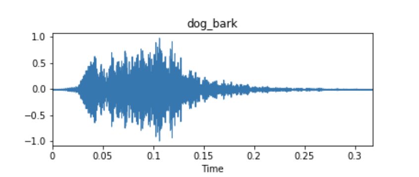
Example waveform of an audio dataset sample from UrbanSound8k.
These audio samples are usually represented as time series, where the y-axis measurement is the amplitude of the waveform. The amplitude is usually measured as a function of the change in pressure around the microphone or receiver device that originally picked up the audio. Unless there is metadata associated with your audio samples, these time series signals will often be your only input data for fitting a model.
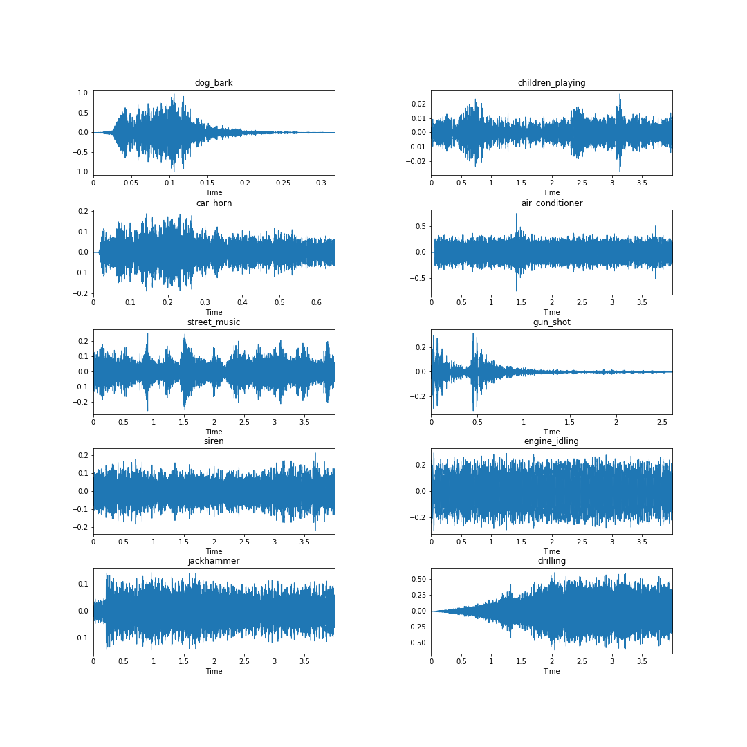
Looking at the samples below, taken from each of the ten classes in the Urbansound8k dataset, it is clear from an eye test that the waveform itself may not necessarily yield clear class identifying information. Consider the waveforms for the engine_idling, siren, and jackhammer classes — they look quite similar.
It turns out one of the best features to extract from audio waveforms (and digital signals in general) has been around since the 1980’s and is still state-of-the-art: Mel Frequency Cepstral Coefficients (MFCCs), introduced by Davis and Mermelstein in 1980. Below we will go through a technical discussion of how MFCCs are generated and why they are useful in audio analysis. This section is somewhat technical, so before we dive in, let’s define a few key terms pertaining to digital signal processing and audio analysis. We’ll link to wikipedia and additional resources if you’d like to dig even deeper.
Disordered Yet Useful Terminology
Sampling and Sampling Frequency
In signal processing, sampling is the reduction of a continuous signal into a series of discrete values. The sampling frequency or rate is the number of samples taken over some fixed amount of time. A high sampling frequency results in less information loss but higher computational expense, and low sampling frequencies have higher information loss but are fast and cheap to compute.
The amplitude of a sound wave is a measure of its change over a period (usually of time). Another common definition of amplitude is a function of the magnitude of the difference between a variable’s extreme values.
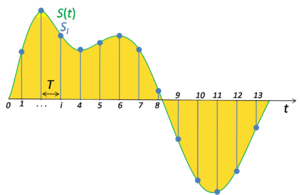
The Fourier Transform decomposes a function of time (signal) into constituent frequencies. In the same way a musical chord can be expressed by the volumes and frequencies of its constituent notes, a Fourier Transform of a function displays the amplitude (amount) of each frequency present in the underlying function (signal).
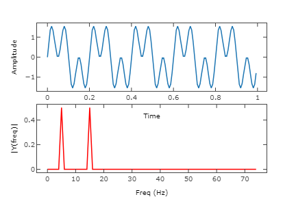
Top: a digital signal; Bottom: the Fourier Transform of the signal.
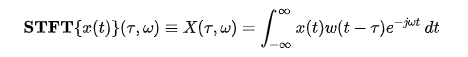
There are variants of the Fourier Transform including the Short-time fourier transform, which is implemented in the Librosa library and involves splitting an audio signal into frames and then taking the Fourier Transform of each frame. In audio processing generally, the Fourier is an elegant and useful way to decompose an audio signal into its constituent frequencies.
*Resources: by far the best video I’ve found on the Fourier Transform is from 3Blue1Brown*
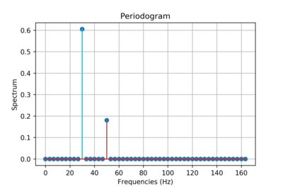
In signal processing, a periodogram is an estimate of the spectral density of a signal. The periodogram above shows the power spectrum of two sinusoidal basis functions of ~30Hz and ~50Hz. The output of a Fourier Transform can be thought of as being (not exactly) essentially a periodogram.
The power spectrum of a time series is a way to describe the distribution of power into discrete frequency components composing that signal. The statistical average of a signal, measured by its frequency content, is called its spectrum. The spectral density of a digital signal describes the frequency content of the signal.
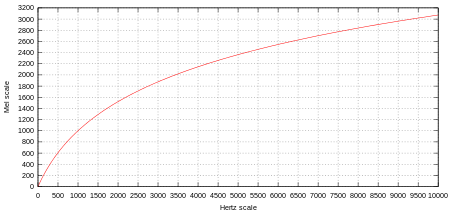
The mel-scale is a scale of pitches judged by listeners to be equal in distance from one another. The reference point between the mel-scale and normal frequency measurement is arbitrarily defined by assigning the perceptual pitch of 1000 mels to 1000 Hz. Above about 500 Hz, increasingly large intervals are judged by listeners to produce equal pitch increments. The name mel comes from the word melody to indicate the scale is based on pitch comparisons.
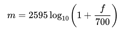
The formula to convert f hertz into m mels is:
The cepstrum is the result of taking the Fourier Transform of the logarithm of the estimated power spectrum of a signal.
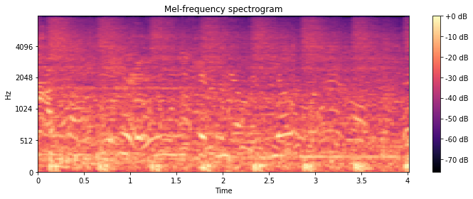
Mel-frequency spectrogram of an audio sample in the Urbansound8k dataset
A spectrogram is a visual representation of the spectrum of frequencies of a signal as it varies with time. A nice way to think about spectrograms is as a stacked view of periodograms across some time-interval digital signal.
The spiral cavity of the inner ear containing the organ of Corti, which produces nerve impulses in response to sound vibrations.
Preprocessing Audio: Digital Signal Processing Techniques
Dataset preprocessing, feature extraction and feature engineering are steps we take to extract information from the underlying data, information that in a machine learning context should be useful for predicting the class of a sample or the value of some target variable. In audio analysis this process is largely based on finding components of an audio signal that can help us distinguish it from other signals.
MFCCs, as mentioned above, remain a state of the art tool for extracting information from audio samples. Despite libraries like Librosa giving us a python one-liner to compute MFCCs for an audio sample, the underlying math is a bit complicated, so we’ll go through it step by step and include some useful links for further learning.
Steps for calculating MFCCs for a given audio sample:
- Slice the signal into short frames (of time)
- Compute the periodogram estimate of the power spectrum for each frame
- Apply the mel filterbank to the power spectra and sum the energy in each filter
- Take the discrete cosine transform (DCT) of the log filterbank energies
Excellent additional reading on MFCC derivation and computation can be found at blog posts here and here.
- Slice the signal into short frames
Slicing the audio signal into short frames is useful in that it allows us to sample our audio into discrete time-steps. We assume that on short enough time scales the audio signal doesn’t change. Typical values for the duration of the short frames are between 20-40ms. It is also conventional to overlap each frame 10-15ms. *Note that the overlapping frames will make the features we eventually generate highly correlated. This is the basis for why we have to take the discrete cosine transform at the end of all of this.*
- Compute the power spectrum for each frame
Once we have our frames we need to calculate the power spectrum of each frame. The power spectrum of a time series describes the distribution of power into frequency components composing that signal. According to Fourier analysis, any physical signal can be decomposed into a number of discrete frequencies, or a spectrum of frequencies over a continuous range. The statistical average of a certain signal as analyzed in terms of its frequency content is called its spectrum.
Source: University of Maryland, Harmonic Analysis and the Fourier Transform
We apply the Short-time fourier transform to each frame to obtain a power spectra for each.
- Apply the mel filterbank to the power spectra and sum the energy in each filter
We still have some work to do once we have our power spectra. The human cochlea does not discern between nearby frequencies well, and this effect only becomes more pronounced as frequencies increase. The mel-scale is a tool that allows us to approximate the human auditory system’s response more closely than linear frequency bands.

Source: Columbia
As can be seen in the visualization above, the mel filters get wider as the frequency increases — we care less about variations at higher frequencies. At low frequencies, where differences are more discernible to the human ear and thus more important in our analysis, the filters are narrow.
The magnitudes from our power spectra, which were found by applying the Fourier transform to our input data, are binned by correlating them with each triangular Mel filter. This binning is usually applied such that each coefficient is multiplied by the corresponding filter gain, so each Mel filter comes to hold a weighted sum representing the spectral magnitude in that channel.
Once we have our filterbank energies, we take the logarithm of each. This is yet another step motivated by the constraints of human hearing: humans don’t perceive changes in volume on a linear scale. To double the perceived volume of an audio wave, the wave’s energy must increase by a factor of 8. If an audiowave is already high volume (high energy), large variations in that wave’s energy may not sound very different.
- Take the discrete cosine transform (DCT) of the log filterbank energies
Because our filterbank energies are overlapping (see step 1), there is usually a strong correlation between them. Taking the discrete cosine transform can help decorrelate the energies.
*****
Thankfully for us, the creators of Librosa have abstracted out a ton of this math and made it easy to generate MFCCs for your audio data. Let’s go through a simple python example to show how this analysis looks in action.
EXAMPLE PROJECT: Urbansound8k + Librosa
We’re going to be fitting a simple neural network (keras + tensorflow backend) to the UrbanSound8k dataset. To begin let’s load our dependencies, including numpy, pandas, keras, scikit-learn, and librosa.
#### Dependencies ####

#### Import Comet for experiment tracking and visual tools
from comet_ml import Experiment
####

import IPython.display as ipd
import numpy as np
import pandas as pd
import librosa
import matplotlib.pyplot as plt
from scipy.io import wavfile as wav

from sklearn import metrics
from sklearn.preprocessing import LabelEncoder

from keras.models import Sequential
from keras.layers import Dense, Dropout, Activation
from keras.optimizers import Adam
from keras.utils import to_categorical
To begin, let’s create a Comet experiment as a wrapper for all of our work. We’ll be able to capture any and all artifacts (audio files, visualizations, model, dataset, system information, training metrics, etc.) automatically.
experiment = Experiment(api_key="API_KEY",
                        project_name="urbansound8k")
Let’s load in the dataset and grab a sample for each class from the dataset. We can inspect these samples visually and acoustically using Comet.
# Load dataset
df = pd.read_csv('UrbanSound8K/metadata/UrbanSound8K.csv')

# Create a list of the class labels
labels = list(df['class'].unique())

# Let's grab a single audio file from each class
files = dict()
for i in range(len(labels)):
    tmp = df[df['class'] == labels[i]][:1].reset_index()
    path = 'UrbanSound8K/audio/fold{}/{}'.format(tmp['fold'][0], tmp['slice_file_name'][0])
    files[labels[i]] = path
We can look at the waveforms for each sample using librosa’s display.waveplot function.
fig = plt.figure(figsize=(15,15))
fig.subplots_adjust(hspace=0.4, wspace=0.4)
for i, label in enumerate(labels):
    fn = files[label]
    fig.add_subplot(5, 2, i+1)
    plt.title(label)
    data, sample_rate = librosa.load(fn)
    librosa.display.waveplot(data, sr= sample_rate)
plt.savefig('class_examples.png')
We’ll save this graphic to our Comet experiment.
# Log graphic of waveforms to Comet
experiment.log_image('class_examples.png')
Next, we’ll log the audio files themselves.
# Log audio files to Comet for debugging
for label in labels:
fn = files[label]
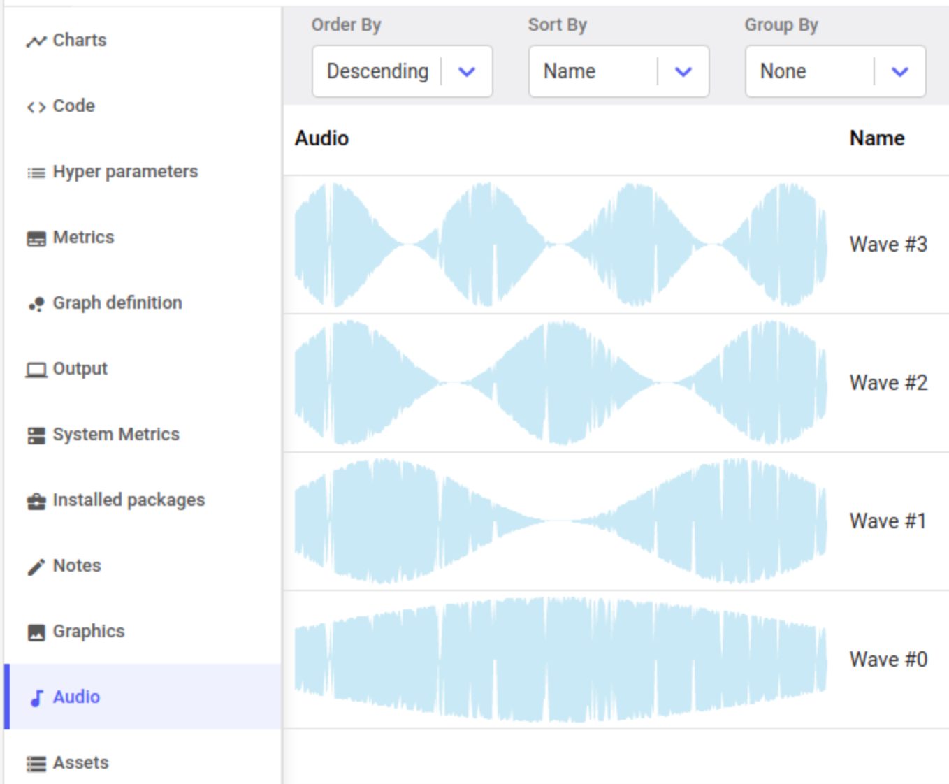
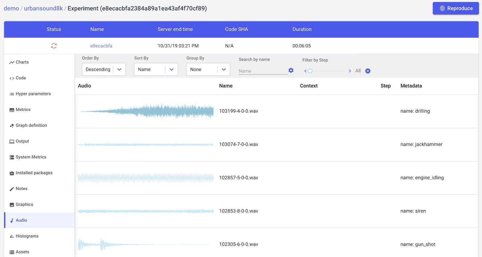
experiment.log_audio(fn, metadata = {'name': label})Once we log the samples to Comet, we can listen to samples, inspect metadata, and much more right from the UI.
Preprocessing
Now we can extract features from our data. We’re going to be using librosa, but we’ll also show another utility, scipy.io, for comparison and to observe some implicit preprocessing that’s happening.
fn = 'UrbanSound8K/audio/fold1/191431-9-0-66.wav'
librosa_audio, librosa_sample_rate = librosa.load(fn)
scipy_sample_rate, scipy_audio = wav.read(fn)

print("Original sample rate: {}".format(scipy_sample_rate))
print("Librosa sample rate: {}".format(librosa_sample_rate))
Original sample rate: 48000
Librosa sample rate: 22050
Librosa’s load function will convert the sampling rate to 22.05 KHz automatically. It will also normalize the bit depth between -1 and 1.
fn = 'UrbanSound8K/audio/fold1/191431-9-0-66.wav'
librosa_audio, librosa_sample_rate = librosa.load(fn)
scipy_sample_rate, scipy_audio = wav.read(fn)

print("Original sample rate: {}".format(scipy_sample_rate))
print("Librosa sample rate: {}".format(librosa_sample_rate))
>Original audio file min~max range: -1869 to 1665
> Librosa audio file min~max range: -0.05 to -0.05
Librosa also converts the audio signal to mono from stereo.
plt.figure(figsize=(12, 4))
plt.plot(scipy_audio)
plt.savefig('original_audio.png')
experiment.log_image('original_audio.png')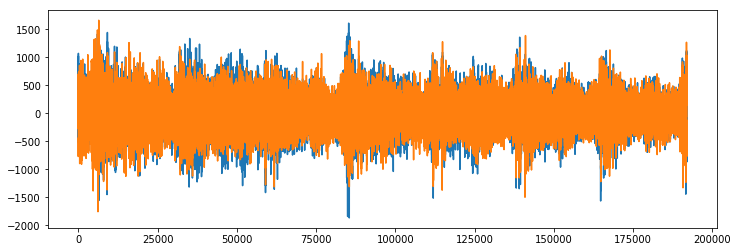
Original Audio (note that it’s in stereo — two audio sources)
plt.figure(figsize=(12, 4))
plt.plot(scipy_audio)
plt.savefig('original_audio.png')
experiment.log_image('original_audio.png')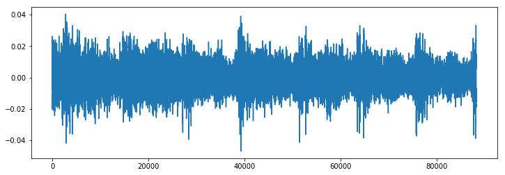
Librosa audio: converted to mono
Extracting MFCCs from audio using Librosa
Remember all the math we went through to understand mel-frequency cepstrum coefficients earlier? Using Librosa, here’s how you extract them from audio (using the librosa_audio we defined above)
mfccs = librosa.feature.mfcc(y=librosa_audio, sr=librosa_sample_rate, n_mfcc = 40)That’s it!
print(mfccs.shape)> (40, 173)
Librosa calculated 40 MFCCs over a 173 frame audio sample.
plt.figure(figsize=(8,8))
librosa.display.specshow(mfccs, sr=librosa_sample_rate, x_axis='time')
plt.savefig('MFCCs.png')
experiment.log_image('MFCCs.png')
MFCC Spectrogram
We’ll define a simple function to extract MFCCs for every file in our dataset.
def extract_features(file_name):    audio, sample_rate = librosa.load(file_name, res_type='kaiser_fast')
    mfccs = librosa.feature.mfcc(y=audio, sr=sample_rate, n_mfcc=40)
    mfccs_processed = np.mean(mfccs.T,axis=0)

    return mfccs_processed
Now let’s extract features.
features = []

# Iterate through each sound file and extract the features
for index, row in metadata.iterrows():

    file_name = os.path.join(os.path.abspath(fulldatasetpath),'fold'+str(row["fold"])+'/',str(row["slice_file_name"]))

    class_label = row["class"]
    data = extract_features(file_name)

    features.append([data, class_label])

# Convert into a Panda dataframe
featuresdf = pd.DataFrame(features, columns=['feature', 'fold' ,'class_label'])
We now have a dataframe where each row has a label (class) and a single feature column, comprised of 40 MFCCs.
featuresdf.head()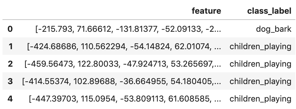
featuresdf.iloc[0]['feature']array([-2.1579300e+02, 7.1666122e+01, -1.3181377e+02, -5.2091331e+01,
-2.2115969e+01, -2.1764181e+01, -1.1183747e+01, 1.8912683e+01,
6.7266388e+00, 1.4556893e+01, -1.1782045e+01, 2.3010368e+00,
-1.7251305e+01, 1.0052421e+01, -6.0095000e+00, -1.3153191e+00,
-1.7693510e+01, 1.1171228e+00, -4.3699470e+00, 7.2629538e+00,
-1.1815971e+01, -7.4952612e+00, 5.4577131e+00, -2.9442446e+00,
-5.8693886e+00, -9.8654032e-02, -3.2121708e+00, 4.6092505e+00,
-5.8293257e+00, -5.3475075e+00, 1.3341187e+00, 7.1307826e+00,
-7.9450034e-02, 1.7109241e+00, -5.6942000e+00, -2.9041715e+00,
3.0366952e+00, -1.6827590e+00, -8.8585770e-01, 3.5438776e-01],
dtype=float32)
Now that we have successfully extracted our features from the underlying audio data, we can build and train a model.
Model building and training
We’ll start by converting our MFCCs to numpy arrays, and encoding our classification labels.
Our dataset will be split into training and test sets. We’ll use the first 8 folds for training and the 9th and 10th folds for testing.
train = feat_df[feat_df['fold'] <= 8]
test = feat_df[feat_df['fold'] > 8]

x_train = np.array(train.feature.tolist())
y_train = np.array(train.class_label.tolist())

x_test = np.array(test.feature.tolist())
y_test = np.array(test.class_label.tolist())

# Encode the classification labels
le = LabelEncoder()
y_train = to_categorical(le.fit_transform(y_train))
y_test = to_categorical(le.fit_transform(y_test))
Let’s define and compile a simple feedforward neural network architecture.
num_labels = y_train.shape[1]
filter_size = 2
def build_model_graph(input_shape=(40,)):
    model = Sequential()
    model.add(Dense(256))
    model.add(Activation('relu'))
    model.add(Dropout(0.5))
    model.add(Dense(256))
    model.add(Activation('relu'))
    model.add(Dropout(0.5))
    model.add(Dense(num_labels))
    model.add(Activation('softmax'))
    # Compile the model
    model.compile(loss='categorical_crossentropy', metrics=['accuracy'], optimizer='adam')

    return model
model = build_model_graph()
Let’s look at a model summary and compute pre-training accuracy.
# Display model architecture summary
model.summary()

# Calculate pre-training accuracy
score = model.evaluate(x_test, y_test, verbose=0)
accuracy = 100*score[1]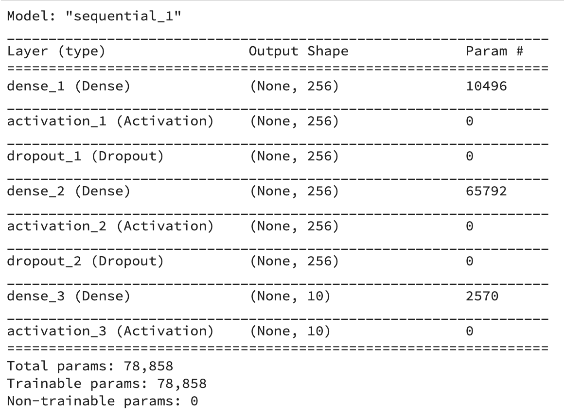
print("Pre-training accuracy: %.4f%%" % accuracy)Pre-training accuracy: 12.2496%
Now it’s time to train our model.
Training completed in time:
from keras.callbacks import ModelCheckpoint
from datetime import datetime

num_epochs = 100
num_batch_size = 32

model.fit(x_train, y_train, batch_size=num_batch_size, epochs=num_epochs, validation_data=(x_test, y_test), verbose=1)
Even before training completed, Comet keeps track of the key information about our experiment. We can visualize our accuracy and loss curves in real time from the Comet UI (note the orange spin wheel indicates that training is in process).
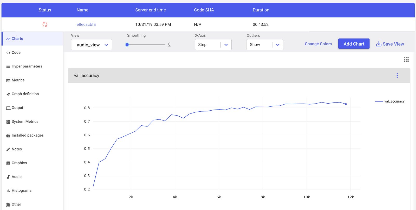
Comet’s Experiment visualization dashboard
Once trained we can evaluate our model on the train and test data.
# Evaluating the model on the training and testing set
score = model.evaluate(x_train, y_train, verbose=0)
print("Training Accuracy: {0:.2%}".format(score[1]))

score = model.evaluate(x_test, y_test, verbose=0)
print("Testing Accuracy: {0:.2%}".format(score[1]))
Training Accuracy: 93.00%
Testing Accuracy: 87.35%
Conclusion
Our model has trained rather well, but there is likely lots of room for improvement, perhaps using Comet’s Hyperparameter Optimization tool. In a small amount of code we’ve been able to extract mathematically complex MFCCs from audio data, build and train a neural network to classify audio based on those MFCCs, and evaluate our model on the test data.
To get started with Comet, click here. Comet is 100% free for public projects.