Natural language processing is a subfield of artificial intelligence that combines computational linguistics, statistics, machine learning, and deep learning models to allow computers to process human language and understand its context, intent, and sentiment.
A generic natural language processing (NLP) model is a combination of multiple mathematical and statistical steps. It usually starts with raw text and ends with a model that can predict outcomes. In between, there are multiple steps that include text cleaning, modeling, and hyperparameter tuning.
Text cleaning, or normalization, is one of the most important steps of any NLP task. It includes removing unwanted data, converting words to their base forms (stemming or lemmatization), and vectorization.
Vectorization is the process of converting textual data into numerical vectors and is a process that is usually applied once the text is cleaned. It can help improve the execution speed and reduce the training time of your code. In this article, we will discuss some of the best techniques to perform vectorization.
Vectorization techniques
There are three major methods for performing vectorization on text data:
1. CountVectorizer
2. TF-IDF
3. Word2Vec
1. CountVectorizer
CountVectorizer is one of the simplest techniques that is used for converting text into vectors. It starts by tokenizing the document into a list of tokens (words). It selects the unique tokens from the token list and creates a vocabulary of words. Finally, a sparse matrix is created containing the frequency of words, where each row represents different sentences and each column represents unique words.
Python’s scikit-learn has a class named CountVectorizer that provides a simple implementation for performing vectorization on text data. Let’s create a sample corpus of food reviews and convert them into vectors using CountVectorizer.
corpus = ['Food is Bad',
          'Bad Service Bad Food',
          'Food is Good',
          'Good Service With Good Food.',
          'Service is Bad but Food is Good.' ]
The first step would be to clean the data by converting text into lowercase and removing stopwords.
import nltk
nltk.download('stopwords')

from nltk.corpus import stopwords
english_stopwords = set(stopwords.words('english'))

corpus = ['Food is Bad',
          'Bad Service Bad Food',
          'Food is Good',
          'Good Service With Good Food.',
          'Service is Bad but Food is Good.']

cleaned_corpus = []
for sent in corpus:
  sent = sent.lower()
  cleaned_corpus.append(' '.join([word for word in sent.split() if word not in english_stopwords]))
print(cleaned_corpus)
cleaned_corpus = ['food bad',
          'bad service bad food',
          'food good',
          'good service good food.',
          'service bad food good.'
         ]
First, we will import the CountVectorizer class:
from sklearn.feature_extraction.text import CountVectorizer
import pandas as pd
vectorizer = CountVectorizer()
X = vectorizer.fit_transform(cleaned_corpus)  ## passing cleaned corpus
doc_term_matrix = pd.DataFrame(X.toarray(),columns= vectorizer.get_feature_names())
print(doc_term_matrix)
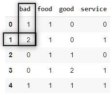
We can easily interpret the Document Term Matrix, which is the output of CountVectorizer. It contains all the unique words and their frequency count in different sentences. For example, the ‘bad’ word count is 2 in the second row because it appeared twice in the second review.
There are also many parameters of CountVectorizer class that can help process the data before applying the vectorization process.
Important parameters of CountVectorizer
lowercase: convert all characters to lowercase.stop_words: remove stopwords from the text before vectorization. {english},list, default=None. If ‘english’, a built-in stop word list is used.strip_accents: {‘ascii’, ‘unicode’}, default=None, Remove accents and perform other character normalization during the preprocessing step.ngram_range: tuple (min_n, max_n), default=(1, 1), range of n-values for different word n-grams to be extracted.
Isolating difficult data samples? Comet can do that. Learn more with our PetCam scenario and discover Comet Artifacts.
2. TF-IDF
TF-IDF or Term Frequency–Inverse Document Frequency, is a statistical measure that tells how relevant a word is to a document. It combines two metrics — term frequency and inverse document frequency — to produce a relevance score.
The Term Frequency is the frequency of a word in a document. It is calculated by dividing the occurrence of a word inside a document by the total number of words in that document.
The Inverse Document Frequency is a measure of how much information a word provides. Words like “the,” for example, occur very frequently but provide little context or value to a sentence. It is calculated by taking the inverse log of document frequency, that is the proportion of documents that contain a particular word.
TF-IDF scores range from 0 to 1. A score closer to 1 is higher the importance of a word to a document.
from sklearn.feature_extraction.text import TfidfVectorizer
Let’s use the same cleaned corpus from the previous example and perform vectorization using TF-IDF.
corpus = ['food bad',
          'bad service bad food',
          'food good',
          'good service good food.',
          'service bad food good.'
         ]
from sklearn.feature_extraction.text import TfidfVectorizer
tf_idf = TfidfVectorizer()
vectors = tf_idf.fit_transform(corpus)
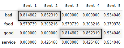
So, according to the TF-IDF algorithm words, ‘bad’ and ‘good’ are the most important words in the whole document, which is some intent to be true. Since, our data contains reviews impact of words that represent a sentiment (good, bad, etc.) tends to be higher.
Unlike a bag of words, TF-IDF not only works upon frequency but also retrieves their importance towards the document.
3. Word2Vec
Word2Vec is a word embedding technique that makes use of neural networks to convert words into corresponding vectors in a way that semantically similar vectors are close to each other in N-dimensional space, where N refers to the dimensions of the vector. This technique was first implemented by Tomas Mikolov at Google back in 2013.
Word2Vec has the ability to maintain semantic relations between words. It can be understood by a simple example where if we have a “king” vector and we remove the vector “man” from the king and add a “women” vector, then we get a vector close to the “queen” vector in N-dimensional space.
king - man + women = queen
There are two ways to implement Word2Vec techniques: Skip-Gram and CBOW, both of which we’ll cover below.
1. Skip-Gram
Skip-Gram tries to predict several context words from a single input word.
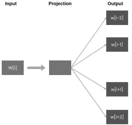
Here w[i] is the input word at position ‘i’ in the sentence. The output of the model contains two preceding words and two succeeding words with respect to location ‘i’.
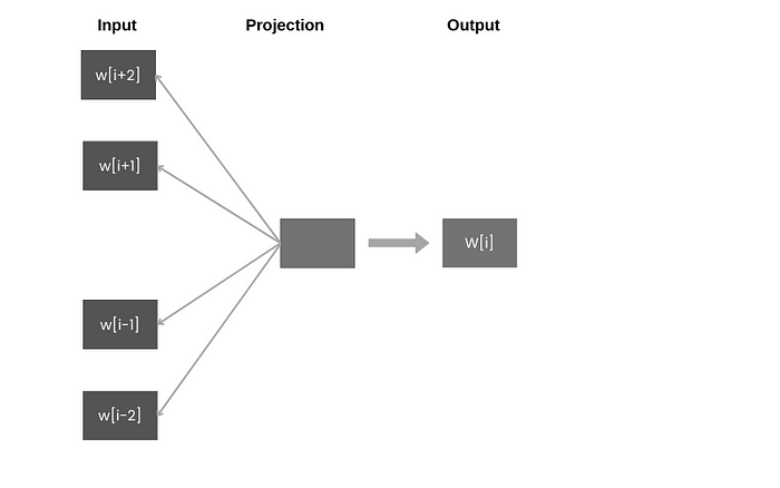
2. CBOW
CBOW stands for Continuous Bag of Words, trained to predict a single word from a series of context words. It is the mirror image of the Skip-Gram technique.
Both techniques are good and can generate vectors from the text by considering semantic similarity. Skip-Gram works well with small-size datasets and can find rare words as well. However, CBOW trains faster and can better represent frequent words. According to the original paper, CBOW takes a few hours to train whereas Skip-Gram needs a few days to understand patterns from the data.
import re
import nltk
from nltk.corpus import stopwords
from nltk.stem import WordNetLemmatizer
wordnet_lemmatizer = WordNetLemmatizer()
## Loading dataset from the github repository raw url
df = pd.read_csv('https://raw.githubusercontent.com/Abhayparashar31/datasets/master/twitter.csv')
## cleaning the text with the help of an external python file containing cleaning function
corpus = []
for i in range(0,len(df)): #we have 1000 reviews
corpus.append(clean_text(df['text'][i])) ## 'clean_text' is a separate python file containing a function for cleaning this data. You can find it here : https://gist.github.com/Abhayparashar31/81997c2e2268338809c46a220d08649f
corpus_splitted = [i.split() for i in corpus]
## Generating Word Embeddings
from gensim import models
w2v = models.Word2Vec(corpus_splitted)
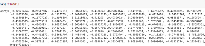
## vector representation of word 'flood'
print(w2v['flood'])
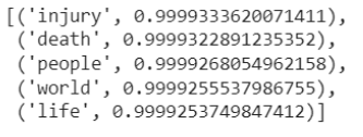
## 5 most similar words for word 'flood'
print(w2v.wv.most_similar('flood')[:5)
The default dimension of word embeddings is 100. we can increase or decrease this number by changing vector_size parameter. You can find more details about different parameters here.
Word2Vec offers different built-in functions to get more insights into the data. most_simiar is one of them that extracts words that have the highest semantic similarity to the input word. Picture 3.4 is a screenshot of the 5 most similar words to the word ‘flood’ based on our data. If we validate the output words [injury, death, people, world, life] are somehow related to ‘flood’. This clearly indicates that our algorithm has done its job.
Recommended readings
1. Efficient Estimation of Word Representations in Vector Space
[word2vec original paper]2. Text Similarity in Vector Space Models: A Comparative Study
[By Omid Shahmirzadi and others]
Conclusion
Vectorization is an important step that is mostly gets ignored by most beginner data scientists. It is a crucial phase of text cleaning that converts your text data into vectors. Later, these vectors are used for training a machine learning algorithm for generating useful predictions. In short, we can say that vectorization is as important as removing unwanted data from the raw text or training an ml model on the data.
