Understanding Memory Mapping in Numpy for Deep Learning: Pt 1
In the previous article, we discussed the possibility of having memory constraints when trying to get into deep learning. I mentioned Numpy’s memory mapping; in this article, we go deeper into the topic and offer an excellent guide to get you started.
There might be a question about why Numpy memory mapping is necessary and who the target demographic is for this particular technique. Now, we can dive into the nitty-gritty details.
Memory-Mapping
Numpy describes its memory mapping feature as accessing small segments of a file without loading the entire file into memory.
This feature highlights the existence of a memory shortage problem for some people. When working with deep learning, arrays might become larger than what could fit in memory. This spells out a problem as it will prevent the computer from running as intended.
Memory mapping will favor someone with access to ample storage compared to memory size (which is often the case). The first step is to save the array as a Numpy binary. Then, from that point onwards, we will load it via memory mapping and perform any operations we deem fit.
Saving Binaries
A binary can easily be described as a file format used to store information. Storing arrays in binaries is convenient as it means you don’t have to waste precious time trying to remake the array whenever you want to return to a problem. A binary allows for easy retrieval of this information whenever needed.
Numpy offers “save()” and “savez()” when you want to save binaries. This functionality is often easy to work with as it has few parameters. You must describe the binary’s path and the array to be stored in binary format. If you have no other needs, then you’re good to go.
For example, if you have an array that stores image data such as training data(X_train and y_train) and you want to store it, you would do the following:
#Splitting training data for image into X and y
X_train = []
y_train = []

for features, labels in training_data:
    X_train.append(features)
    y_train.append(labels)

#Saving into a binary
from numpy import save

save("X_train.npy", X_train)
save("y_train.npy", y_train)
The above code snippet will save one binary each for the X_train array and the y_train array, respectively.
Once the binary file is saved, there are multiple ways to load the file into memory to perform operations. The standard method involves just loading them as they are into memory. The second way requires memory mapping.
Loading Binaries
Numpy offers a few tools to load binaries as desired. The first method is by using “load()” while the second is using “memmap().” There are advantages and disadvantages to using each one.
The first method allows someone to use memory mapping or load directly, as efficiently and fluidly as possible. The only difference is an argument away.
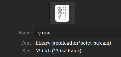
I made two binary files to perform this example and to show how load() works. The first binary is a 1.4 GB file we will memory map, and the second is a 32 KB file that will be entirely loaded into memory.


from numpy import load

#Load binary as y_train
y_train = load("y_train.npy)
Running the above code will call the entirety of y_train into memory, and we can check this using the “sys” library. We expect it to occupy a memory amount similar to the storage size.
import sys

#checking the size of the file in memory
print(f'y_train memory occupied: {sys.getsizeof(y_train)} bytes')

It has occupied 32 KB, as we expected it to. We have demonstrated what loading into memory does and expect it to behave similarly if a different, larger file is loaded. This is where our memory mapping comes into the picture, as we can load a smaller amount of content into memory.
The “X_train” file is 1.4 GB, but only a tiny fraction of the memory will be occupied when we alter the code we wrote.
from numpy import load
import sys

#Loads the X_train.npy
X_train = load("X_train.npy", mmap_mode='r')
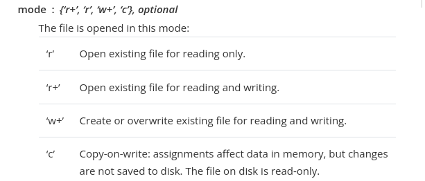
Here, we include the “mmap_mode” argument and choose “r” as our preferred mode. It refers to read-only and is one of four modes that are offered. All the modes are as defined below in the Numpy documentation:

Now, we can perform a similar test to the previous one and check how much memory X_train will use after using the memory-mapped mode.
print(f'X_train memory occupied: {sys.getsizeof(X_train)} bytes')

Impressively enough, our much larger file now occupies significantly less memory when memory-mapped. It only occupies 184 bytes but remains in a format that could be used for tasks such as training models or tasks like predicting labels without much additional overhead.
#model fitting will work just as usual with memory-mapped variables

model.fit(X_train, y_train)

#predicting will also similarly be the same
y_predict = model.predict(X_test)
Disclaimer
This method is not a magic bullet for all your problems, as there are a few things to remember when using memory mapping.
One consideration is whether you want to operate on the loaded binary. If you desire to work on the memory-mapped file, it will become an array and occupy the memory you set out to save. It is, therefore, advisable to split the data into slices to iterate on any given operation.
Another consideration is the modes offered when using “mmap_mode()”. If the binary needs changes, then the appropriate mode may not be the default mode that only supports read-only.
Wrap Up…
Memory mapping is a great way to save memory when performing operations that may occupy a lot of space. In this article, we learned how to use Numpy’s “load()” to load things entirely into the memory and how to perform memory mapping.
Numpy also offers “memmap()” for this particular job, but it has different dynamics that we will explore in the second part of this article.


