ResNet: How One Paper Changed Deep Learning Forever
In December of 2015 a paper was published that rocked the deep learning world.
Widely regarded as one of the most influential papers in modern deep learning, it has been cited over 110,000 times. The name of this paper will go down in the annals of deep learning history: Deep Residual Learning for Image Recognition (aka, the ResNet paper).
This paper showed the deep learning community that it was possible to construct increasingly deeper network architectures that can either perform well or at least the same as the shallower networks.
When AlexNet hit the scene in 2012, prevailing wisdom suggested adding more layers to neural networks would lead to better results. This was evidenced by breakthroughs coming from VGGNet, GoogleNet, and others.
This set the deep learning community on a quest to go deeper.
It turns out, though, that learning better networks is not as easy as stacking more and more layers. Researchers observed that the accuracy of deep networks would increase up to a saturation point before leveling off. Additionally, an unusual phenomenon was observed:
Training error would increase as you add layers to an already deep network.
This was primarily due to two problems
1) Vanishing/exploding gradients
2) The degradation problem
Vanishing/exploding gradients

The vanishing/exploding gradients problem is a by-product of the chain rule. The chain rule multiplies error gradients for weights in the network. Multiplying lots of values that are less than one will result in smaller and smaller values. As those error gradients approach the earlier layers of a network, their value will tend to zero.
This results in smaller and smaller updates to earlier layers (not much learning happening).
The inverse problem is the exploding gradient problem. This occurs due to large error gradients accumulating during training, resulting in massive updates to model weights in the earlier layers (since multiplying lots of values that are bigger than 1 will result in larger and larger values).
The reason for this issue?
Parameters in earlier layers of the network are far away from the cost function, which is the source of the gradient that is propagated backward through the network. As the error is back propagated through an increasingly deep network, a larger number of parameters contribute to the error. The net result of both of these scenarios is that early layers in the network become more difficult to train.
But there’s another more curious problem…
The degradation problem
Adding more and more layers to these deep models leads to higher training errors, ending in a degradation in the expressive power of your network.
The degradation problem is unexpected, because its not caused by overfitting. Researchers were finding that as networks got deeper, the training loss would decrease but then shoot back up as more layers were added to the networks. Which is counterintuitive because you’d expect your training error to decrease, converge, and plateau out as the number of layers in your network increases.

Let’s imagine that you had a shallow network that was performing well.
If you take a “shallow” network and just stack on more layers to create a deeper network, the performance of the deeper network should be at least as good as the shallow network. Why? Because, in theory, deeper network could learn the shallow network. The shallow network is a subset of the deeper network. But this doesn’t happen in practice!
You could even set the new stacked layers to be identity layers, and still find your training error getting worse when you stack more layers on top of a shallower model. Deeper networks were leading to higher training error!
Both of these issues — the vanishing/exploding gradients and degradation problems — threatened to halt progress of deep neural networks, until the ResNet paper came out.
The ResNet paper introduced a novel solution to these two pesky problems that plagued the architects of deep neural networks.
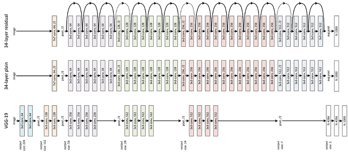
The skip connection

Skip connections, which are housed in residual blocks, allow you to take the activation value from an earlier layer and pass it to a deeper layer in a network. Skip connections enable deep networks to learn the identity function. Learning the identity function allows a deeper layer to perform as well as an earlier layer, or at the very least it won’t perform any worse. The result is smoother gradient flow, ensuring important features are preserved in the training process.
The invention of the skip connection has given us the ability to build deeper and deeper networks while avoiding the problem of vanishing/exploding gradients and degradation.
Here’s how it works…

Instead of the previous layers output being passed directly onto the next block, a copy of that output is made, then that copy is passed through a residual block. This residual block will process the copied output matrix, X — with a 3×3 convolution, followed by batch norm and ReLU to yield a matrix Z.
Then, X and Z would be added together, element by element, to yield the output to the next layer/block.

Doing this helps us ensure that any added layers in a neural network are useful for learning. Worst case scenario is that the residual block could output a bunch of zeros, which leaves the X+Z to end up still being X, since X+Z=X if Z is just the zero matrix.
ResNet in action!
Now it’s time to see ResNet in action.
You could try to implement ResNet from scratch, train it on ImageNet, and try to find the optimal training parameters yourself… but why do that when you can use something out of the box? That’s what SuperGradients gives you: A pre-trained ResNet model with a robust set of training parameters that is ready for you to use with minimal configuration!
You’ll learn a bit about transfer learning and how to use the SuperGradientstraining library on the MiniPlaces dataset to perform image classification. SuperGradients is a PyTorch based training library that has pre-trained models for classification, detection, and segmentation tasks.
You can follow along here, or open up this notebook on Google Colab to get hands on:
Install dependencies
You’ll need to install the following dependencies.
!pip install super_gradients==3.0.0 gwpy &> /dev/null
!pip install matplotlib==3.1.3 &> /dev/null
!pip install torchinfo &> /dev/null
Import packages
Now you can import all the packages necessary for this tutorial.
import os
import requests
import zipfile
import random
import numpy as np
import torchvision
import pprint
import torch
import pathlib

from matplotlib import pyplot as plt
from torchinfo import summary
from pathlib import Path, PurePath
from torchvision import transforms
from torchvision import datasets
from torch.utils.data import DataLoader
from PIL import Image
from typing import List, Tuple
import super_gradients
from super_gradients.training import models
from super_gradients.training import dataloaders
from super_gradients.training import Trainer
from super_gradients.training import training_hyperparams
Download data
You’ll use use miniplaces dataset. You can learn more about the dataset here.
torchvision.datasets.utils.download_and_extract_archive('https://dissect.csail.mit.edu/datasets/miniplaces.zip','datasets')
Configurations
The following class houses configuration values that will be helpful as you progress along the tutorial.
class config:
    EXPERIMENT_NAME = 'resnet_in_action'
    MODEL_NAME = 'resnet50'
    CHECKPOINT_DIR = 'checkpoints'

    # specify the paths to training and validation set
    TRAIN_DIR = 'datasets/miniplaces/train'
    VAL_DIR = 'datasets/miniplaces/val'

    # set the input height and width
    INPUT_HEIGHT = 224
    INPUT_WIDTH = 224

    # set the input height and width
    IMAGENET_MEAN = [0.485, 0.456, 0.406]
    IMAGENET_STD = [0.229, 0.224, 0.225]

    NUM_WORKERS = os.cpu_count()

    DEVICE = 'cuda' if torch.cuda.is_available() else 'cpu'

    FLIP_PROB = 0.25
    ROTATION_DEG = 15
    JITTER_PARAM = 0.25
    BATCH_SIZE = 64
Experiment setup
When working with SuperGradients first thing you have to do is initialize your trainer.
The trainer is in charge of pretty much everything from training, evaluation, saving checkpoints, plotting etc. The experiment name argument is important as all checkpoints, logs and tensorboards will be saved in a directory with the same name.
This directory will be created as a sub-directory of ckpt_root_dir as follow:
ckpt_root_dir
|─── experiment_name_1
│       ckpt_best.pth                     # Model checkpoint on best epoch
│       ckpt_latest.pth                   # Model checkpoint on last epoch
│       average_model.pth                 # Model checkpoint averaged over epochs
│       events.out.tfevents.1659878383... # Tensorflow artifacts of a specific run
│       log_Aug07_11_52_48.txt            # Trainer logs of a specific run
└─── experiment_name_2
        ...
trainer = Trainer(experiment_name=config.EXPERIMENT_NAME, ckpt_root_dir=config.CHECKPOINT_DIR, device=config.DEVICE)
Create dataloaders
The SG trainer is compatible with PyTorch dataloaders, so you can use your own dataloaders.
def create_dataloaders(
    train_dir: str,
    val_dir: str,
    train_transform: transforms.Compose,
    val_transform:  transforms.Compose,
    batch_size: int,
    num_workers: int=config.NUM_WORKERS
):
  """Creates training and validation DataLoaders.
  Args:
    train_dir: Path to training data.
    val_dir: Path to validation data.
    transform: Transformation pipeline.
    batch_size: Number of samples per batch in each of the DataLoaders.
    num_workers: An integer for number of workers per DataLoader.
  Returns:
    A tuple of (train_dataloader, val_dataloader, class_names).
  """
  # Use ImageFolder to create dataset
  train_data = datasets.ImageFolder(train_dir, transform=train_transform)
  val_data = datasets.ImageFolder(val_dir, transform=val_transform)

  print(f"[INFO] training dataset contains {len(train_data)} samples...")
  print(f"[INFO] validation dataset contains {len(val_data)} samples...")

  # Get class names
  class_names = train_data.classes
  print(f"[INFO] dataset contains {len(class_names)} labels...")

  # Turn images into data loaders
  print("[INFO] creating training and validation set dataloaders...")
  train_dataloader = DataLoader(
      train_data,
      batch_size=batch_size,
      shuffle=True,
      num_workers=num_workers,
      pin_memory=True,
  )
  val_dataloader = DataLoader(
      val_data,
      batch_size=batch_size,
      shuffle=False,
      num_workers=num_workers,
      pin_memory=True,
  )

  return train_dataloader, val_dataloader, class_names
Transforms
This next code block will instantiate a transformation pipeline for both training and validation.
# initialize our data augmentation functions
resize = transforms.Resize(size=(config.INPUT_HEIGHT,config.INPUT_WIDTH))

horizontal_flip = transforms.RandomHorizontalFlip(p=config.FLIP_PROB)

vertical_flip = transforms.RandomVerticalFlip(p=config.FLIP_PROB)

rotate = transforms.RandomRotation(degrees=config.ROTATION_DEG)

norm = transforms.Normalize(mean=config.IMAGENET_MEAN, std=config.IMAGENET_STD)

make_tensor = transforms.ToTensor()

# initialize our training and validation set data augmentation pipeline
train_transforms = transforms.Compose([resize, horizontal_flip, vertical_flip, rotate, make_tensor, norm])
val_transforms = transforms.Compose([resize, make_tensor, norm])
Instantiate dataloaders
Now you can instantiate your dataloaders.
train_dataloader, valid_dataloader, class_names = create_dataloaders(train_dir=config.TRAIN_DIR,
                                                                     val_dir=config.VAL_DIR,
                                                                     train_transform=train_transforms,
                                                                     val_transform=val_transforms,
                                                                     batch_size=config.BATCH_SIZE)

NUM_CLASSES = len(class_names)
Some heuristics for transfer learning
1) Your dataset is small and similar to the dataset the model was pre-trained on.
When your images are similar its likely that low-level features (like edges) and high-level features (like shapes) will be similar.
What to do: Freeze the weights up to last layer, replace the fully connected layer, and retrain. Why? Less data means you can overfit if you train the entire network.
Comet Artifacts lets you track and reproduce complex multi-experiment scenarios, reuse data points, and easily iterate on datasets. Read this quick overview of Artifacts to explore all that it can do.
2) Your dataset is large and similar to the dataset the model was pre-trained on.
What to do: Freeze the earlier layer weights. Then retain later weights with a new fully connected layer.
3) Your dataset is small and different from the dataset the model was pre-trained on.
This is the most difficult situation to deal with. The pre-trained network is already finely-tuned at each layer. You don’t want any of the high-level features and you can’t afford to retrain because you run the risk of overfitting.
What to do: Remove the fully connected layers and convolutional layers closer to the output. Retrain the convolutional layers closer to the input.
4) Your dataset is large and different from the dataset the model was pre-trained on.
You should instantiate the pre-trained model weights to speed up training (lot’s of the low-level convolutions will have similar weights).
What to do: Retrain the entire network from scratch, making sure to replace the fully connected output layer.
To train ResNet from scratch in SG all you need to do is omit the pretrained_weights="imagenet" argument from the models.get method.
For this example, we will go with option 2.
Instantiate your ResNet model
Using SuperGradients makes changing the classification head of your model simple. All you have to do is pass in the number of classes for your use case to the num_classes argument and the classification head will automatically be changed for you.
resnet50_imagenet_model = models.get(model_name=config.MODEL_NAME, num_classes=NUM_CLASSES, pretrained_weights="imagenet")
This next block of code will freeze the early layers and batch norm layers of the instantiated model.
for param in resnet50_imagenet_model.conv1.parameters():
    param.requires_grad = False

for param in resnet50_imagenet_model.bn1.parameters():
    param.requires_grad = False

for param in resnet50_imagenet_model.layer1.parameters():
    param.requires_grad = False

for param in resnet50_imagenet_model.layer2.parameters():
    param.requires_grad = False
Training setup
The training parameters in SuperGradients were optimized per dataset and architecture with consideration for the type of training used(from scratch\transfer learning).
For more recommended training params you can have a look at our recipes here.
You won’t need to tune hyperparamters in this example, but you are more than welcome to play around with some!
training_params =  training_hyperparams.get("training_hyperparams/imagenet_resnet50_train_params")

#overriding the number of epochs to train for
training_params["max_epochs"] = 3
Training and evaluation
The results of the training epochs are kept in your CKPT path that was defined. Let’s go ahead and train the model.
You’ll notice a few metrics displayed for each epoch:
AccuracyLabelSmoothingCrossEntropyLossTop5
Let’s define the two that you may not be familiar with.
LabelSmoothingCrossEntropyLoss.
In classification problems, sometimes our model learns predict the training examples extremely confidently. This is not good for generalization. Label smoothing is a regularization technique for classification problems that prevent a model from predicting the training examples too confidently. This is used to increase robustness for classification problems.
Top5
Top-5 accuracy means one of the model’s top 5 highest probability predictions match the ground truth. If it does, you count it as a correct prediction.
To train your model all you have to do is run the following code:
trainer.train(model=resnet50_imagenet_model,
              training_params=training_params,
              train_loader=train_dataloader,
              valid_loader=valid_dataloader)

# Load the best model that we trained
best_model = models.get(config.MODEL_NAME,
                        num_classes=NUM_CLASSES,
                        checkpoint_path=os.path.join(trainer.checkpoints_dir_path,"ckpt_best.pth"))
Let’s see how well our model predicts on the validation data
Now that the model is trained you can examine how well it predicts on validation data. This next block of code will predict on images from the validation set.
# 1. Take in a trained model, class names, image path, image size, a transform and target device
def pred_and_plot_image(model: torch.nn.Module,
                        image_path: str,
                        class_names: List[str],
                        image_size: Tuple[int, int] = (config.INPUT_HEIGHT, config.INPUT_WIDTH),
                        transform: torchvision.transforms = None,
                        device: torch.device=config.DEVICE):


    # 2. Open image
    if isinstance(image_path, pathlib.PosixPath):
      img = Image.open(image_path)
    else:
      img = Image.open(requests.get(image_path, stream=True).raw)

    # 3. Create transformation for image (if one doesn't exist)
    if transform is not None:
        image_transform = transform
    else:
        image_transform = transforms.Compose([
            transforms.Resize(image_size),
            transforms.ToTensor(),
            transforms.Normalize(mean=config.IMAGENET_MEAN,
                                 std=config.IMAGENET_STD),
        ])

    ### Predict on image ###

    # 4. Make sure the model is on the target device
    model.to(device)

    # 5. Turn on model evaluation mode and inference mode
    model.eval()
    with torch.inference_mode():
      # 6. Transform and add an extra dimension to image (model requires samples in [batch_size, color_channels, height, width])
      transformed_image = image_transform(img).unsqueeze(dim=0)

      # 7. Make a prediction on image with an extra dimension and send it to the target device
      target_image_pred = model(transformed_image.to(device))

    # 8. Convert logits -> prediction probabilities (using torch.softmax() for multi-class classification)
    target_image_pred_probs = torch.softmax(target_image_pred, dim=1)

    # 9. Convert prediction probabilities -> prediction labels
    target_image_pred_label = torch.argmax(target_image_pred_probs, dim=1)

    #actual label
    ground_truth = PurePath(image_path).parent.name

    # 10. Plot image with predicted label and probability
    plt.figure()
    plt.imshow(img)
    if isinstance(image_path, pathlib.PosixPath):
      plt.title(f"Ground Truth: {ground_truth} | Pred: {class_names[target_image_pred_label]} | Prob: {target_image_pred_probs.max():.3f}")
    else:
      plt.title(f"Pred: {class_names[target_image_pred_label]} | Prob: {target_image_pred_probs.max():.3f}")
    plt.axis(False);

# Get a random list of image paths from test set
num_images_to_plot = 30
test_image_path_list = list(Path(config.VAL_DIR).glob("*/*.jpg")) # get list all image paths from test data
test_image_path_sample = random.sample(population=test_image_path_list, # go through all of the test image paths
                                       k=num_images_to_plot) # randomly select 'k' image paths to pred and plot

# Make predictions on and plot the images
for image_path in test_image_path_sample:
    pred_and_plot_image(model=best_model,
                        image_path=image_path,
                        class_names=class_names,
                        image_size=(config.INPUT_HEIGHT, config.INPUT_WIDTH))
Now that the training is complete you can use the trained model to predict on an unseen image!
Let’s see what place the model thinks this image is:

pred_and_plot_image(model=best_model,
                    image_path="https://cdn.pastemagazine.com/www/articles/2021/05/18/the-office-NEW.jpg",
                    class_names=train_dataloader.dataset.classes,
                    image_size=(config.INPUT_HEIGHT, config.INPUT_WIDTH))
If you enjoyed this tutorial and think SuperGradients is a cool tool to use, then consider giving it a star on on GitHub. Looking for a community of deep learning practitioners? Then hang out at the Deep Learning Daily community, where deep learning practitioners come to learn new skills and solve their most difficult problems.
Related Articles