
Introduction
Have you ever questioned how we can become so engrossed in watching videos on YouTube and how some of these posts end up on your Facebook or Instagram timeline? For those of us who are familiar with Netflix, we frequently receive recommendations for movies that are similar to the ones we are looking for or perhaps the ones we have just finished watching. This is made possible by an algorithm known as the “recommendation system.” In this tutorial, we’ll talk more about the recommendation system, build a system for recommending movies, and then integrate it into Comet.
Recommendation Systems
There are 3 main types of Recommendation systems
- Content-Based Recommendation system.
- Popularity-Based Recommendation system.
- Collaborative Recommendation system.
Content-Based Recommendation system:
It is a type of recommendation system that operates on a similar content principle. If a user is watching a movie, the system will look for other movies with similar content or in the same genre as the one the user is watching. When comparing similar content, various fundamental attributes are used to compute similarity.
Popularity-Based Recommendation System:
It is a type of recommendation system that operates based on popularity of anything that is currently popular. These systems examine the products or movies that are popular among users and directly recommend them.
For instance, if a product is frequently purchased by the majority of people, the system will learn that it is the most popular, so for every new user who has just signed up, the system will recommend that product to that user as well, and the chances are that the new user will also purchase that.
Collaborative Recommendation system
Collaborative recommendation, also called collaborative filtering, works by analyzing the preferences and data of numerous users. Collaborative filtering predicts a user’s interests. This is accomplished by applying techniques involving cooperation among numerous agents, data sources, etc. to filter data for information or patterns. The underlying premise of collaborative filtering is that users A and B are likely to have similar tastes in products if they have similar tastes in one product.
Comet
Comet is a platform for experimentation that enables you to monitor your machine-learning experiments. Comet has another noteworthy feature: it allows us to conduct exploratory data analysis. We can accomplish our EDA objectives thanks to Comet’s integration with well-known Python visualization frameworks. You can learn more about comet here.
This lesson will teach us how to connect Comet with our recommendation system. We will carry out some EDA on our movie dataset to achieve this, and we will log the visualization onto the Comet experimentation website or platform. Let’s begin without further ado.
Prerequisites
You may install the Comet library on your computer if you don’t already have it there by using the following line at the command prompt.
pip install comet_ml
— or —
conda install -c comet_ml
About the data
All 45,000 films mentioned in the Full MovieLens Dataset are represented by these files’ information. Movies that were released on or before July 2017 are included in the dataset. Cast, crew, narrative keywords, budget, revenue, posters, release dates, language breakdowns, production firms, nations, and TMDB vote counts and averages are just a few examples of the data points.
Additionally, this collection includes files with 26 million user ratings for all 45,000 movies, collected from 270,000 individuals. A scale of 1 to 5 stars was used to rate each item on the GroupLens official website. You can get the data from Kaggle here.
Real-time model analysis allows your team to track, monitor, and adjust models already in production. Learn more lessons from the field with Comet experts.
Movie Recommendation system
The first step involves importing the dependencies.
import numpy as np
import pandas as pd
import seaborn as sns
import matplotlib.pyplot as plt
import difflib
from sklearn.feature_extraction.text import TfidfVectorizer
from sklearn.metrics.pairwise import cosine_similarity
We then move to load our dataset into the pandas dataframe.
movie_data = pd.read_csv('/content/jmovies.csv')
We then move to the next step, which is data preprocessing.
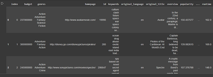
movie_data.head()
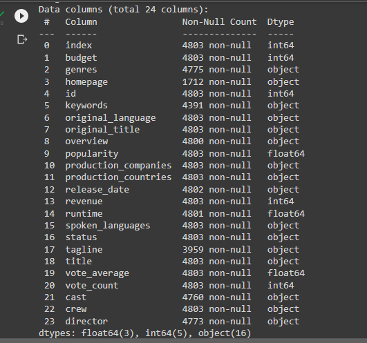
movie_data.info()
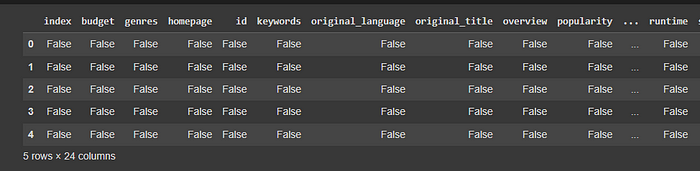
movie_data. isnull()
The movie_data. isnull() function returns false if the values in the dataset are not missing and return true if they are missing.
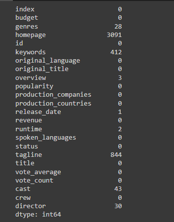
The movie_data. isnull().head() function only gives us the details on the first 5 columns, but to know the exact column and how many values are missing, we use the movie_data. isnull().sum() function tells us which column has missing values and the number of missing values it has.
movie_data. isnull().sum()
We have a lot of elements in our dataset and not all can be used for our recommendation system, so we select only those that can be used. We also pick elements that will affect the accuracy of our recommendation system. Users are most likely to watch a movie based on the class of genres, the type of cast in the movie, and also the director in charge of the movie
From our data preprocessing, we can see that we have a lot of missing values in our dataset, which will affect the result of our recommendation system. We need to fill it up with null strings, but before we do that, we need to perform some EDA.
movie_data[['keywords','tagline','cast','director']].fillna('')
We then create a variable named “combined features” input all the selected features and print them. This is done so we can input it as a whole into our vectorizer, which converts the text to feature vectors.
combined_features= movie_data['genres']+' '+movie_data['keywords'] \
+' '+movie_data['tagline']+' '+movie_data['cast'] \
+' '+movie_data['director']
The next step involves converting our text data to numerical data and this is done so it can be understood by the cosine similarity, which works well with numerical data we be using TfidfVectorizer to convert.
vectorizer = TfidfVectorizer()
feature_vectors = vectorizer.fit_transform(combined_features)
So once the numerical data is ready, we then try and get the similarity scores using cosine similarity, and we then load our feature vector into the cosine similarity to find movies that are similar to each other. So what the cosine similarity does is iterate through the list and try to find similarities between the selected character and the remaining movies in the dataset, it does this for each of the movies.
similarity = cosine_similarity(feature_vectors)print(similarity)
print(similarity.shape)
To get our recommendation system working we need to create an input section for the user to input the name of their selected movie.
movie_name = input(' Enter your favourite movie name : ')
We then need to create a list of the names of all movies in the dataset.
list_of_all_titles = movie_data['title'].tolist()
print(list_of_all_titles)
The next step is finding a movie match for the movie name that the user inputs.
find_close_match = difflib.get_close_matches(movie_name,
                                             list_of_all_titles)
print(find_close_match)
The above code gives us a list of related movies but we need to narrow it down to the exact movie the user inputs.
close_match = find_close_match[0]
print(close_match)
To get the index of each movie we use the title of the movie to find the index
index_of_the_movie = movie_data[movie_data.title == close_match]['index'].values[0]
print(index_of_the_movie)
So, using the index value, we will be getting a list of similar values. So when you run this code you’ll notice the index of the movie.
similarity_score = list(enumerate(similarity[index_of_the_movie]))
print(similarity_score)
We then print the length of the similarity score.
len(similarity_score)
We then sort the movie based on the similarity score. So the same genres of movies are sorted together.
sorted_similar_movies = sorted(similarity_score, key = lambda x:x[1], reverse = True)
print(sorted_similar_movies)
Then we work on printing a list based on the similarity scores.
print('Movies suggested for you : \n')i = 1for movie in sorted_similar_movies:
    index = movie[0]
    title_from_index = movies_data[movies_data.index==index]['title'].values[0]
    if (i<30):
        print(i, '.',title_from_index)
        i+=1
So we can see that our recommendation system is up and running and the movie’s recommendation works just fine. So the next step includes logging our visualization on the comet platform.
So we need to visualize some of the characters in our dataset using matplotlib and seaborn.
mask_df = movie_data["director"].value_counts().head(10)
fig1 = plt.figure(figsize=(12, 10))
plt.bar(x = mask_df.index, height=mask_df, color="sienna")
plt.xlabel("director")
plt.ylabel("budget")
plt. title("Budget of each director per movie")
plt.xticks(rotation=45)
So the above code shows the budget of each director per movie and we can see how the budget for each movie varies per director.
In the next step, we input the budget per movie, and we can see which of the movies has the highest budget.
fig2 = plt.figure(figsize=(12, 10))
sns.histplot(movie_data["budget"], color="darkslategrey", bins=50)
plt.title("Budget of Movie");
The next step will be to log the visualization onto the Comet platform once we have finished it. In this section, we’ll use the Comet experiment library to build a brand-new project.
You will require a Comet API key to continue with this phase. Click here to sign up for their platform if you haven’t already. By clicking on your profile photo, selecting the settings icon, and then scrolling down, as demonstrated below, you can find your API key.

from comet_ml import Experiment# Create an experiment with your API keyexperiment = Experiment(
api_key="xGZbEEC8bB2VnpxWFcWXd3BI3",
project_name="Recommendation system",
workspace="olujerry",
)
experiment.log_figure(figure_name="Matplotlib Viz", figure=fig1)
experiment.log_figure(figure_name= "Seaborn Viz", figure=fig2)
We imported the Experiment library from comet ml into the code above. We then instantiated it and assigned it to the experiment variable. Your API key, the name of your project, and the name of your workspace are some of the parameters needed by the Experiment library. The Comet platform will display the workspace name, such as:
experiment.log_figure(figure_name="Matplotlib Viz", figure=fig1)experiment.log_figure(figure_name= "Seaborn Viz", figure=fig2)experiment.end()
To log our visualization to the Comet Platform, use the two lines of code above. Seaborn Visualization and Matplotlib both use the.log figure()methods. Then we give our visualization a name.
Recall that we previously gave our visualizations the names fig1 and fig2, which we then pass to the figure parameter.
If you are using a notebook, such as Jupyter or Colab, you must type the experiment.end () after your test.
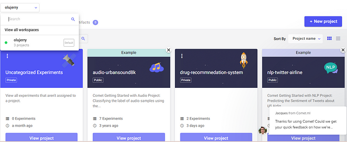
We can now view our experiments on the project session on the website.
Conclusion
This article taught us how to incorporate our recommendation system into Comet. The majority of Python libraries for data science and machine learning are integrated with Comet. Check out some additional datasets that can be used to enhance the recommendation engine. The full code used in this tutorial can be found here.
