Conventionally, doctors use magnetic resonance imaging (MRI) scans to help with the diagnosis of various medical conditions such as cancer. However, in certain cases, accurate diagnosis cannot be performed based on the images alone. For instance, glioblastoma, the most common form of brain cancer, has an analysis procedure that involves the extraction of a tissue sample from the patient through surgery. Moreover, the characterization of the tumor can take weeks. So, a computer-aided solution is welcome to aid doctors in not only producing more accurate diagnoses but providing them at a faster rate.
Deep learning has been successful in solving computer vision problems. This method has been extended to the medical field. In this article, I will show you how to build a classifier that predicts the presence of a tumor from MRI scans. I will be using the data from the RSNA-MICCAI Brain Tumor Radiogenomic Classification competition hosted by Kaggle. For the implementation, I will be referencing the top solution of the competition, which can be found in this repository.
Understanding the Data
We are given a training dataset with a folder structure of this:
train
|---00000
    |---FLAIR
        |Image-1.dcm
        |Image-1.dcm
        |...
    |---T1w
    |---T1wCE
    |---T2w
|---00001
|---00002
|---...
This means that for each patient ID (such as “00000”), we are given 4 different cases or scans obtained from different pulse sequences. In each case, there are DICOM files that have a format of .dcm . From the additional CSV file provided to us, each patient ID is mapped to a binary value that signifies the presence of the brain tumor.
DICOM files
DICOM stands for “Digital Imaging and Communications in Medicine.” It is a standard, internationally accepted format to view, store, retrieve, and share medical images. Typically, a special medical DICOM viewer needs to be installed to access DICOM files. Luckily, we can use the PyDicom package that allows us to read the files in Python. We can do this using the read_filefunction:
dicom = pydicom.read_file(path)
If we print out the dicom object, we will be shown the metadata. Some elements of the metadata are useful for understanding the data we are dealing with. Let’s inspect them.
Metadata
Rows and columns: These parameters define the image size. Their values are both 512. So, each image size has a size of 512 pixels by 512 pixels.
Samples per pixel: Defines the number of color channels. The value of 1 here means the image is grayscale.
Photometric interpretation: The value is “MONOCHROME2,” meaning the image is grayscale and a pixel value of 0 indicates a black pixel. This is the opposite of “MONOCHROME1,” where a pixel value of 0 indicates a white pixel. Hence, knowing the value of this metadata is important, or it will affect our image processing.
Pixel spacing: Indicates the physical distance between the centers of each pixel in mm. The value shown is [0.5, 0.5], which means the physical distances between each pixel in both x and y directions are both 0.5 mm.
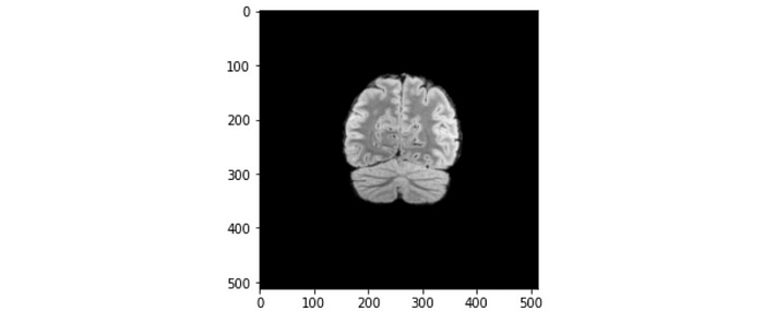
Let’s apply this piece of information to one of the brain slices. Referring to the figure above, the maximum length across the brain slice is approximately 200 pixels, which translates to 200 x 0.5 mm = 100 mm = 10 cm. The length of 10 cm makes sense for a normal brain size.
Series description: For each patient, we are provided with 4 different folders of DICOM files, namely “FLAIR,” “T1w,” “T1wCE,” and “T2W.” These are scans obtained using different MRI pulse sequences. An MRI pulse sequence is a programmed set of changing magnetic gradients. Each sequence is defined by multiple parameters, such as time to echo (TE), time to repetition (TR), inversion pulse, and diffusion weighting. Different combinations of these parameters affect tissue contrast and spatial resolution. We can make use of this piece of information to decide what to do with the data. We can choose to include every pulse sequence in a single dataset, or train the model separately on different pulse sequences.
Bits allocated: Defines the amount of space allocated for every sample in bits. Not all allocated bits are used to define the pixel value. Hence, the bits stored (0028,0101) can be fewer than the bits allocated. In our case, they are both 16 bits. This means it has a pixel range of 2¹⁶ = 65536. However, the 8-bit monitor which we typically use can only display 256 shades of gray. What radiologists normally do is windowing. Windowing allows us to view the part of the brain that is more relevant for diagnosis. By adjusting two parameters called the window center and window width, we are able to accentuate the appearance of different components of the brain, such as bone, soft tissues, water, fat, lung, and air.
Window center and window width: This is for the purpose of windowing. For instance, if the window center and window width are 71 and 142, respectively, then:
- The lowest visible pixel value = 71 -(142/2) = 0
- The highest visible pixel value = 71-(142/2) =142
The pixel values between 0 and 142 are displayed as-is. Any pixel value below 0 will show up as black, whereas any pixel value above 142 will show up as white.
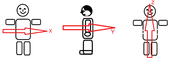
Patient orientation: It is [1, 0, 0, 0, 0, -1] for every file. It should be read as two separate vectors: [1, 0, 0] and [0, 0, -1], which represent x-axis and the negative z-axis, respectively. The coordinate system and the directions of XYZ axes are illustrated in the figure below.
Let us compare the image position of the first and the last DICOM file of the patient with the ID “00000.”
Image position of the first DICOM file: [-125.094, 90.3865, 127.74]
Image position of the last DICOM file: [-125.094, -137.013, 127.74]
The y-coordinate value decreases while the other two coordinates remain the same. According to the coordinate system defined by DICOM, it implies that the scans were performed along the y-axis from the back of the head to the front of the head. To further confirm this, let us analyze the orientation of each DICOM image.
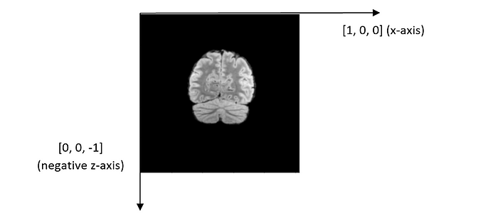
From the coordinate system above, we can infer that we are viewing the brain image from the patient’s front, with the forehead facing us.
The most important thing to keep in mind when building and deploying your model? Understanding your end-goal. Read our interview with ML experts from Stanford, Google, and HuggingFace to learn more.
Data Processing
We now understand the data we are given. For each patient, each DICOM file contains an image of a cross-section of the brain taken from the posterior to the anterior. We can combine these images into a 3-dimensional array structure that represents a brain before sending it to the model to output a binary prediction of whether or not the tumor exists.
Read a DICOM file and extract the image array. Then, we can choose to apply windowing using the apply_voi_lut function provided in the PyDicom package.
def load_dicom_image(path, img_size=256, voi_lut=True, rotate=0):
    dicom = pydicom.read_file(path)
    data = dicom.pixel_array
    if voi_lut:
        data = apply_voi_lut(arr=dicom.pixel_array, ds=dicom)
    else:
        data = dicom.pixel_array

    data = cv2.resize(data, (img_size, img_size))
    data -= np.min(data)
    if np.min(data) < np.max(data):  # to prevent zero division
        data /= np.max(data)

    return data
Let us inspect some of the images. What we are seeing here are cross-sections (slices) of a brain.

We then create a PyTorch Dataset.
class BrainRSNADataset:
    def __init__(...):
        (...)  # removed for brevity purposes

    def __getitem__(self, index):
        row = self.data.loc[index]
        case_id = int(row.BraTS21ID)
        target = int(row[self.target])
        _3d_images = self.load_dicom_images_3d(case_id)
        _3d_images = torch.tensor(_3d_images).float()
        if self.is_train:
            return {"image": _3d_images, "target": target, "case_id": case_id}
        else:
            return {"image": _3d_images, "case_id": case_id}

    def load_dicom_images_3d(self, case_id, num_imgs=64, img_size=256, rotate=0):
        """Outputs a 3D numpy array from the 2D images of each case"""
        case_id = str(case_id).zfill(5)  # adds zeros (0) at the beginning of the string
        s = "rsna-miccai-brain-tumor-radiogenomic-classification"
        path = f"../input/{s}/{self.folder}/{case_id}/{self.type}/*.dcm"
        files = sorted(
            glob.glob(path),
            key=lambda var: [int(x) if x.isdigit() else x for x in re.findall(r"[^0-9]|[0-9]+", var)]
        )

        middle = self.img_indexes[case_id]  # the window centre is the biggest image
        num_imgs2 = num_imgs // 2
        p1 = max(0, middle - num_imgs2)  # beginning of 3D image
        p2 = min(len(files), middle + num_imgs2)
        image_stack = [load_dicom_image(f, rotate=rotate, voi_lut=True) for f in files[p1:p2]]
        img3d = np.stack(image_stack).T  # flip between first and last dimension.

        # Add zeros matrices to make the last dim to have a length of `num_imgs`
        if img3d.shape[-1] < num_imgs:
            n_zero = p.zeros((img_size, img_size, num_imgs - img3d.shape[-1]))
            img3d = np.concatenate((img3d, n_zero), axis=-1)

        return np.expand_dims(img3d, 0)
Now, there is a slight problem with creating a 3-dimensional representation of the image. First of all, the number of slices for every DICOM image is different. Besides, due to computation costs, we might need to limit the number of slices sent to the model.
One solution that is intuitive and straightforward is to select the middle nnumber of slices. However, this might not be the ideal solution. This is because the middle slice might not be the exact center of the brain. The solution author offered a better solution: obtain the slice that has the largest brain area, then grab the (n-1)/2 slices before and after it. This solution assumes the slice with the largest brain area is the center of the brain. According to the solution author, it did help him get better performance.
def _prepare_biggest_images(self):
    big_image_indexes = {}
    for row in tqdm(self.data.iterrows(), total=len(self.data)):
        case_id = str(int(row[1].BraTS21ID)).zfill(5)
        path = f"../input/{self.folder}/{case_id}/{self.type}/*.dcm"
        files = sorted(
          glob.glob(path),
          key=lambda var: [int(x) if x.isdigit() else x for x in re.findall(r"[^0-9]|[0-9]+", var)]
        )
        resolutions = [extract_cropped_image_size(f) for f in files]
        middle = np.array(resolutions).argmax()  # Select the image with the largest brain slice
        big_image_indexes[case_id] = middle
    return big_image_indexes
Model
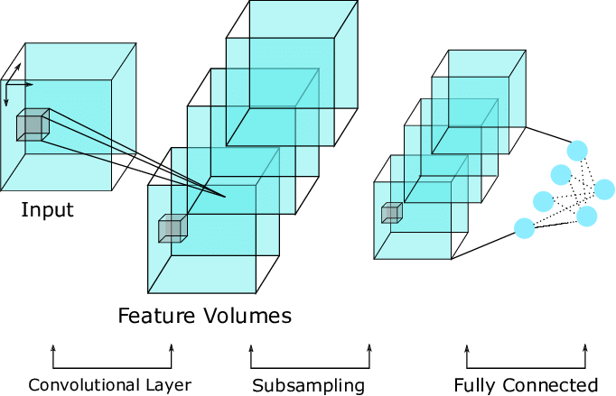
For 2D images, we use a 2-dimensional convolutional neural network as the deep learning model. This is no longer applicable in our case since our images are now represented in 3 spatial dimensions. Instead, we use a 3-dimensional convolutional neural network (3D CNN). The concept is similar to 2D CNNs, just that the kernel filter slides in 3 dimensions instead of 2.
To create a 3D CNN, we are going to use the MONAI framework. MONAI is a freely available, community-supported, PyTorch-based framework for deep learning in healthcare imaging. It supports a lot of modules and utilities catered for this purpose. We can use a pre-trained model such as ResNet-10 using just one line of code:
model = monai.networks.nets.resnet10(
    spatial_dims=3, n_input_channels=1, n_classes=1
)
The model is trained similarly as one would with 2D CNNs. Since we have a binary classification problem, we can use binary cross-entropy loss. The training loop is similar to the one we normally use. The solution author used Adam as the optimizer with a learning rate of 1e-4. The scheduler is MultiStepLR , which decays the learning rate of each parameter group by gamma once the number of epoch reaches one of the milestones.
optimizer = optim.Adam(model.parameters(), lr=0.0001)
scheduler = lr_scheduler.MultiStepLR(optimizer, milestones=[10], gamma=0.5, last_epoch=-1, verbose=True)
model.zero_grad()
criterion = nn.BCEWithLogitsLoss()

for counter in range(config.N_EPOCHS):
    epoch_iterator_train = tqdm(train_dl)
    tr_loss = 0.0
    for step, batch in enumerate(epoch_iterator_train):
        model.train()
        images, targets = batch["image"].to(device), batch["target"].to(device)
        outputs = model(images)
        loss = criterion(outputs.squeeze(1), targets.float())
        loss.backward()
        optimizer.step()
        model.zero_grad()
        optimizer.zero_grad()
        tr_loss += loss.item()
        epoch_iterator_train.set_postfix(batch_loss=(loss.item()), loss=(tr_loss / (step + 1)))
    scheduler.step()
This approach got the solution author top of the leaderboard, with an AUROC score of 0.62174. However, the solution author acknowledges that the leaderboard is rather noisy, and judging from the relatively low AUROC score (just slightly above 0.5), I believe that more data will help improve the performance.
Conclusion
In this article, we learned about DICOM files for medical images and how to interpret the metadata. By doing so, we understand how the data are obtained, and thus we are able to make informed decisions about how the data should be represented. In addition, we also learned about representing a 3-dimensional brain structure using a series of 2D images. By combining these techniques, we can certainly get at least a good baseline model for a classification task on MRI-based medical data.
However, this is by no means a replacement for actual doctors because deep learning models lack interpretability no matter how good they can be. Consider this, if a computer diagnoses you of brain cancer without telling you how it comes up with this prediction, how much will you trust its judgment? I certainly would be skeptical! Therefore, it might be wise for computer vision to act as a tool to further aid doctors’ diagnosis rather than work toward replacing them completely.
