Debugging Classifiers with Confusion Matrices
Introduction
A confusion matrix is a visual way to inspect the performance of a classification model. Metrics such as accuracy can be inadequate in cases where there are large class imbalances in the data, a problem common in machine learning applications for fraud detection. A confusion matrix can provide us with a more representative view of our classifier’s performance, including which specific instances it is having trouble classifying.
In this post we are going to illustrate two ways in which Comet’s confusion matrix can help debug classification models.
For our first example, we will run an experiment similar to the one illustrated in this post on imbalanced data. We’re going to train a classifier to detect fraudulent transactions in an imbalanced dataset and use Comet’s confusion matrix to evaluate our model’s performance. In our second example we will cover classification on unstructured data with a large number of labels using the CIFAR100 dataset and a simple CNN model.
Confusion Matrices with Imbalanced Data
In this example, we’re going to use the Credit Card Fraud Detection dataset from Kaggle to evaluate our classifier. This dataset is highly imbalanced, with only 492 fraudulent transactions present in a dataset with 284,807 transactions in total. Our model is a single fully connected layer with Dropout enabled. We’re going to train our model using the Adam optimizer for 5 epochs, with a batch size of 64 and use 20% of our dataset for validation.
def load_data():
    raw_df = pd.read_csv(
        "https://storage.googleapis.com/download.tensorflow.org/data/creditcard.csv"
    )

    return raw_df

def preprocess(raw_df):
    df = raw_df.copy()

    eps = 0.01

    df.pop("Time")
    df["Log Ammount"] = np.log(df.pop("Amount") + eps)

    train_df, val_df = train_test_split(df, test_size=0.2)

    train_labels = np.array(train_df.pop("Class"))
    val_labels = np.array(val_df.pop("Class"))

    train_features = np.array(train_df)
    val_features = np.array(val_df)

    scaler = StandardScaler()
    train_features = scaler.fit_transform(train_features)
    val_features = scaler.transform(val_features)

    train_features = np.clip(train_features, -5, 5)
    val_features = np.clip(val_features, -5, 5)

    return train_features, val_features, train_labels, val_labels
|
Training a classifier
Our model is a single fully connected layer with Dropout enabled. We’re going to train our model using the Adam optimizer for 5 epochs, with a batch size of 64 and use 20% of our dataset for validation.
def build_model(input_shape, output_bias=None):
    if output_bias is not None:
        output_bias = tf.keras.initializers.Constant(output_bias)
    model = keras.Sequential(
        [
            keras.layers.Dense(16, activation="relu", input_shape=(input_shape,)),
            keras.layers.Dropout(0.5),
            keras.layers.Dense(1, activation="sigmoid", bias_initializer=output_bias),
        ]
    )

    model.compile(
        optimizer=keras.optimizers.Adam(lr=1e-3),
        loss=keras.losses.BinaryCrossentropy(),
        metrics=["accuracy"],
    )

    return model
|
Since we’re using Keras as our modelling framework, Comet will automatically log our hyperparameters, and training metrics (accuracy and loss) to the web UI. At the end of every epoch we’re going to log a confusion matrix of the model’s predictions on our validation dataset using a custom Keras callback and Comet’s `log_confusion_matrix` function.
class ConfusionMatrixCallback(Callback):
    def __init__(self, experiment, inputs, targets, cutoff=0.5):
        self.experiment = experiment
        self.inputs = inputs
        self.cutoff = cutoff
        self.targets = targets
        self.targets_reshaped = keras.utils.to_categorical(self.targets)

    def on_epoch_end(self, epoch, logs={}):
        predicted = self.model.predict(self.inputs)
        predicted = np.where(predicted < self.cutoff, 0, 1)

        predicted_reshaped = keras.utils.to_categorical(predicted)
        self.experiment.log_confusion_matrix(
            self.targets_reshaped,
            predicted_reshaped,
            title="Confusion Matrix, Epoch #%d" % (epoch + 1),
            file_name="confusion-matrix-%03d.json" % (epoch + 1),
        )

def main():
    experiment = Experiment(workspace=WORKSPACE, project_name=PROJECT_NAME)

    df = load_data()
    X_train, X_val, y_train, y_val = preprocess(df)

    confmat = ConfusionMatrixCallback(experiment, X_val, y_val)
    model = build_model(input_shape=X_train.shape[1])
    model.fit(
        X_train,
        y_train,
        validation_data=(X_val, y_val),
        epochs=5,
        batch_size=64,
        callbacks=[confmat],
    )
|
Results
We see that our model is able to achieve a very high validation accuracy after a single epoch of training. This is misleading, since only 0.17% of the dataset has a positive label. We can achieve over 99% accuracy on this dataset by simply predicting a 0 label for any given transaction.
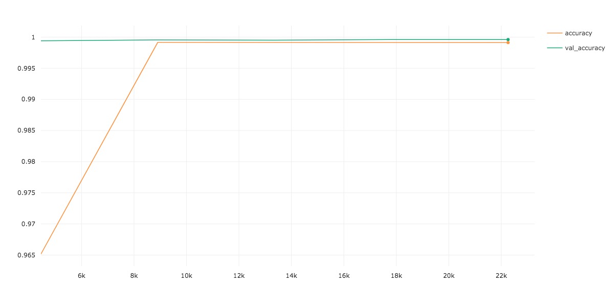
Let’s take a look at our Confusion Matrix to see what our real performance is like.
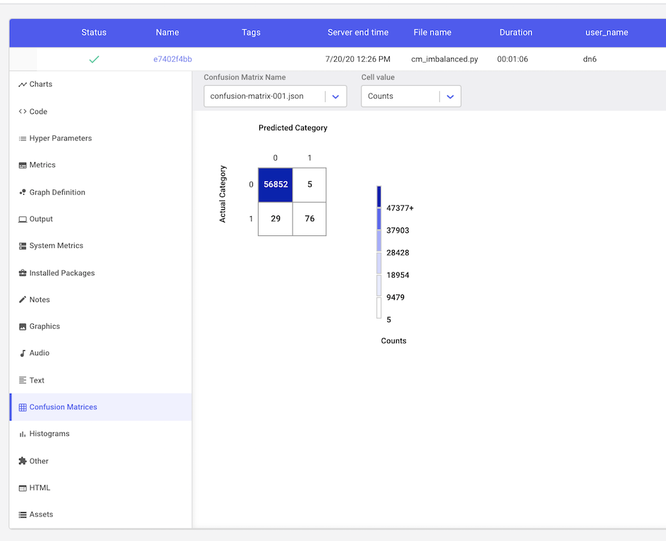
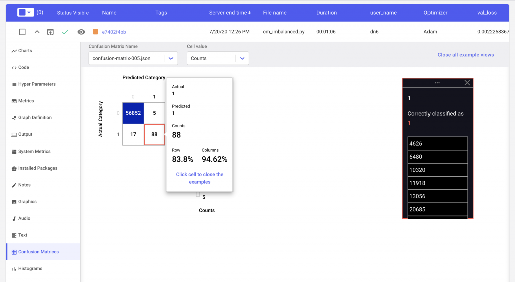
For our binary classification task, we see that after a single epoch of training our model produces 5 false positive and 29 false negative predictions. If our classifier was perfect, these values would be 0. By clicking on the cell with the false negatives, we can see the indices in our validation dataset that were incorrectly classified as not fraudulent.
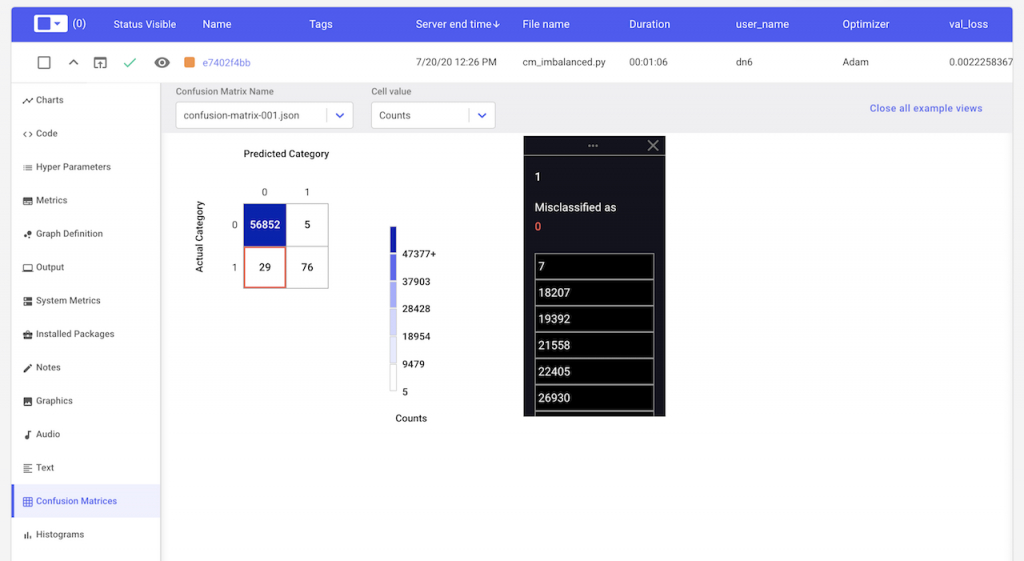
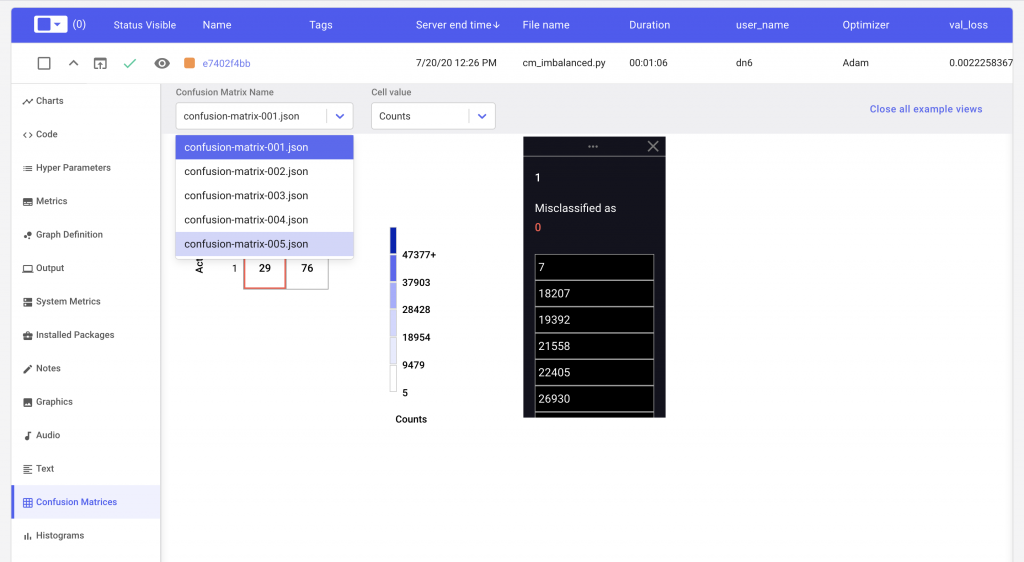
We can also see if our predictions improved over time by changing the epoch number in the dropdown selector.
Lastly, in order to get an estimate of the per class performance, we can simply hover over the cell corresponding to that class. In Figure 5, we see that our classifier’s accuracy when it comes to detecting a true fraudulent transaction is closer to 83% rather than the reported validation accuracy of 99%.
Comet Confusion Matrix with Unstructured Data
Comet makes it easy to deal with classification problems that depend on unstructured data. We’re going to use the CIFAR100 dataset and a simple CNN to illustrate how the ConfusionMatrix callback is used for these types of data.
First, let’s fetch our dataset, and preprocess it using the built in convenience methods in Keras
# Load CIFAR-100 data
(input_train, target_train), (input_test, target_test) = cifar100.load_data()# Parse numbers as floats
input_train = input_train.astype("float32")
input_test = input_test.astype("float32")

# Normalize data
input_train = input_train / 255
input_test = input_test / 255

target_train, target_test = tuple(
map(lambda x: keras.utils.to_categorical(x), [target_train, target_test])
)
|
Next, we’ll define our CNN architecture for this task as well as our training parameters, such as batch size and number of epochs.
# Model configuration batch_size = 128 img_width, img_height, img_num_channels = 32, 32, 3 loss_function = categorical_crossentropy no_classes = 100 no_epochs = 100 optimizer = Adam() verbosity = 1 validation_split = 0.2 interval = 10 # Build the Model model = Sequential() model.add(Conv2D(128, kernel_size=(3, 3), activation="relu", input_shape=input_shape)) model.add(MaxPooling2D(pool_size=(2, 2))) model.add(Conv2D(128, kernel_size=(3, 3), activation="relu")) model.add(MaxPooling2D(pool_size=(2, 2))) model.add(Conv2D(64, kernel_size=(3, 3), activation="relu")) model.add(MaxPooling2D(pool_size=(2, 2))) model.add(Flatten()) model.add(Dense(256, activation="relu")) model.add(Dense(128, activation="relu")) model.add(Dense(no_classes, activation="softmax")) |
Finally, we’ll update our Confusion Matrix callback from the previous example so that we use a single Confusion Matrix object for the entire training process. This updated callback will only create a confusion matrix every Nth epoch, where N is controlled by the interval parameter.
class ConfusionMatrixCallback(keras.callbacks.Callback):
    def __init__(self, experiment, inputs, targets, interval):
        self.experiment = experiment
        self.inputs = inputs
        self.targets = targets
        self.interval = interval

        self.confusion_matrix = ConfusionMatrix(
            index_to_example_function=self.index_to_example,
            max_examples_per_cell=5,
            labels=LABELS,
        )

    def index_to_example(self, index):
        image_array = self.inputs[index]
        image_name = "confusion-matrix-%05d.png" % index
        results = experiment.log_image(image_array, name=image_name)
        # Return sample, assetId (index is added automatically)
        return {"sample": image_name, "assetId": results["imageId"]}

    def on_epoch_end(self, epoch, logs={}):
        if (epoch + 1) % self.interval != 0:
            return
        predicted = self.model.predict(self.inputs)
        self.confusion_matrix.compute_matrix(self.targets, predicted)
        self.experiment.log_confusion_matrix(
            matrix=self.confusion_matrix,
            title="Confusion Matrix, Epoch #%d" % (epoch + 1),
            file_name="confusion-matrix-%03d.json" % (epoch + 1),
        )
|
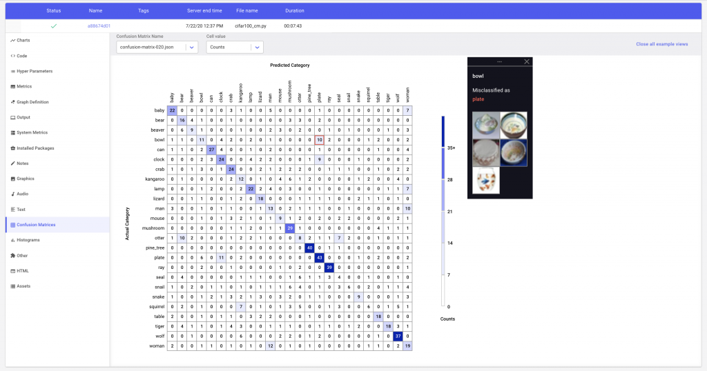
Using a single instance of the Confusion Matrix ensures that the fewest number of images are logged to Comet as it reuses them wherever possible over all epochs of training. These uploaded examples will be available inside our Confusion Matrix in the UI, and allow us to easily view the specific instances that our model is having difficulty classifying.
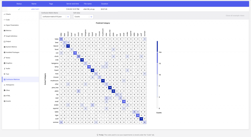
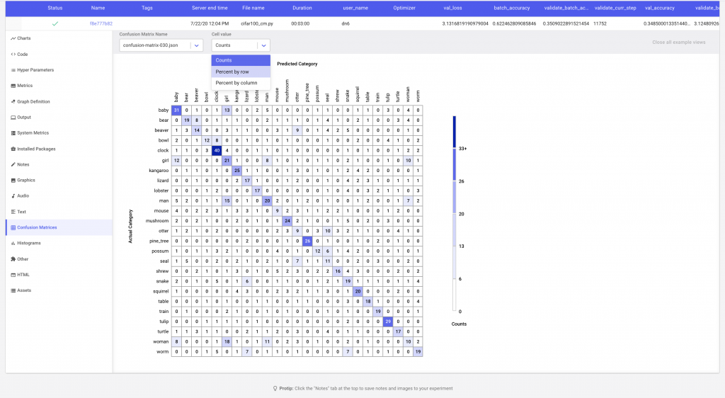
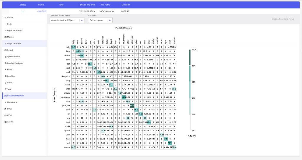
In Figure 6 we see that the Comet confusion matrix has trimmed down the total number of classes to the ones that the model is most confused about. i.e. the labels with the most misclassifications. By clicking on a cell, we can see examples of instances that have been misclassified. We can also change the what values are displayed in each cell of the matrix by changing the cell value to show the percent of correct predictions by row or column.
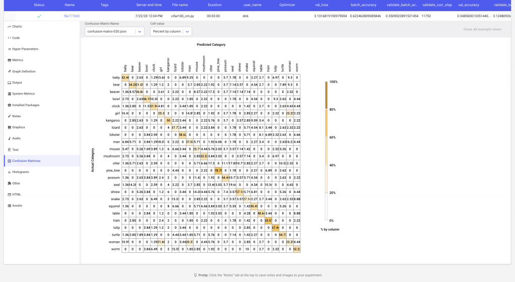
In this example, Comet’s Confusion Matrix will upload the image examples as assets to the experiment. Alternatively, if your images are hosted somewhere else, or you are using assets such as audio, Comet’s confusion matrix can map the index of the classified example to the url of the corresponding asset.
The Confusion Matrix API also allows the user to control the number of assets uploaded to Comet. We can either specify the maximum number of examples to be uploaded per cell, or provide a list of the classes that we are interested in comparing to the selected argument in the Confusion Matrix constructor.
Conclusion
In this post, we’ve gone through an example of a classification task where our target data is highly imbalanced. We’ve shown how a metric like accuracy cannot accurately capture the true performance of our model and why visual tools like the confusion matrix can help us get a more granular understanding of our model performance across different classes.
You can also explore the experiment on imbalanced data in more detail:
Comet Experiment for Imbalanced Data: Get access to the code used to generate these results on here.
Colab Notebook for Imbalanced Data: If you would like to run the code yourself, you can test it out in a Colab Notebook here. Keep in mind that you will need a Comet account and a Comet API Key to run the notebook.
We also demonstrated how Comet’s confusion matrix can be configured to work with unstructured data, and how it can provide examples of misclassified labels for easy model debugging.
Comet Experiment for CIFAR100: All the code necessary to reproduce these results can be found here
Colab Notebook for CIFAR100: here. We would recommend enabling the GPU on the notebook before running it. You can do this by navigating to Edit→Notebook Settings, and selecting GPU from the Hardware Accelerator drop-down.
*Note:* Comet’s Confusion Matrix also supports R. Check out the example here
Want to stay in the loop? Subscribe to the Comet Newsletter for weekly insights and perspective on the latest ML news, projects, and more.
Related Articles

